QuickGraph#16 The English WordNet in Neo4j (part 1)

English WordNet is a representation of the English language a lexical network. It groups words into synsets and links them according to semantic relationships such as hypernymy, antonymy and meronymy. You can actually browse through its content from the English Wordnet website. Wordnet is often used in natural language processing (NLP) applications (but also many others) and provides deep lexical information about the English language as a graph. As a graph… that sounds interesting, definitely worth a QuickGraph.

Because this is a particularly rich case I’ll break it down in at least two instalments. In the first one I’ll explain the construction of the graph in Neo4j and in the second one I’ll show some interesting ways of using it. I hope you’ll enjoy it.

Building the Graph in Neo4j

This section describes in detail how to build the English Wordnet graph in Neo4j. If you don’t care about this you can probably jump to the next one where I explore the resulting graph or maybe come back next week for part 2 of this QuickGraph where we’ll look at different ways of using the English Wordnet graph.

Data Ingestion: Importing the RDF dump

A full export of the English WordNet is published annually by the Global Wordnet Association and you can download it here in a number of formats that include RDF (Turtle).

As you know Neo4j can import RDF datasets in a fully automated manner through the neosemantics (n10s) plugin. All you would need to do is download the .gz file from the previous link and import it into Neo4j with the following single line of code:

CALL n10s.rdf.import.fetch(".../english-wordnet-2020.ttl.gz","Turtle");

This would import the 3.1 million triples in the dataset and create a graph with roughly 1 million nodes and 2 million relationships. As a reference, I’ll share that in my machine (a relatively modern MBP) the import takes approximately 55 seconds.

At this point you would be ready to start using the graph but I’ve decided to apply a few changes to it, and refactor some modelling patterns that are OK(ish) in RDF but that you definitely want to avoid in a Property Graph, let’s look at a couple of them (note: what I’m about to explain is very similar to what I did in this QuickGraph on the Thomson Reuters PermId dataset).

The script for the whole import process (the data ingestion plus the refactorings that we are about to cover now) can be found here. You can copy it and run it directly on your Neo4j instance to get the final version of the WordNet graph.

Node To Label refactoring: Part of Speech nodes

Let’s start by having a look at the POS (part of speech) nodes. There are five of them: noun, verb, adverb, adjective and adjective_satellite and there are tens of thousands of both Lexical entries and lexical concepts linking to them through the partOfSpeech relationship. You can get a summary of this with this query:

match ()-[:wn__partOfSpeech]->(pos) 
return pos.uri, count(*)

which produces the following results:

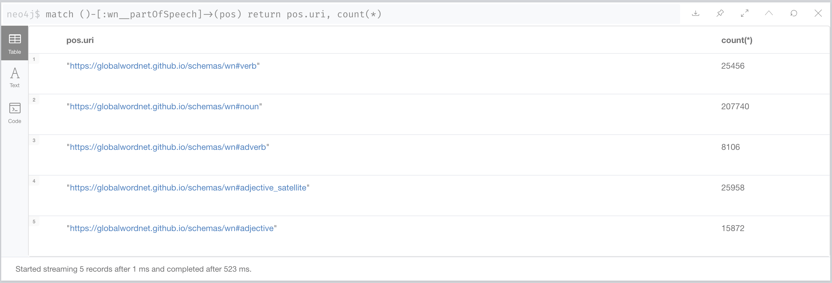
In the Property Graph model we have labels to classify nodes and in this particular case they are a much more efficient mechanism to “tag” a node (both lexical entries and lexical concepts) with their POS. The following image captures visually the refactoring that we are about to carry out:

And this is the cypher fragment that does the job for lexical entries (with a little bit of help from APOC).

MATCH (le:ontolex__LexicalEntry)-[:wn__partOfSpeech]->(pos)
WITH le, apoc.text.join([x in split(apoc.text.replace(pos.uri,".*#(.*)$","$1"),"_") | apoc.text.capitalize(x)],"") AS posAsString
SET le.wn__partOfSpeech = posAsString
WITH le, posAsString
CALL apoc.create.addLabels(le, [n10s.rdf.shortFormFromFullUri("http://www.lexinfo.net/ontology/2.0/lexinfo#" + posAsString)]) yield node
RETURN count(node)

Removing super-dense nodes: Single lexicon node

You will notice that all lexical concepts and lexical entries (nearly 300K in total) are linked through the entry relationship to a single node representing the lexicon to indicate that they are part of it. This dense node is not very useful particularly in this context where I’m working with a single lexicon in my DB so I’ll remove it along with all of its nearly 300000 relationships.

You can use this query to do it:

match (r:Resource { uri: "https://en-word.net/"}) detach delete r 

Node to property refactoring: Lexical Concept definitions

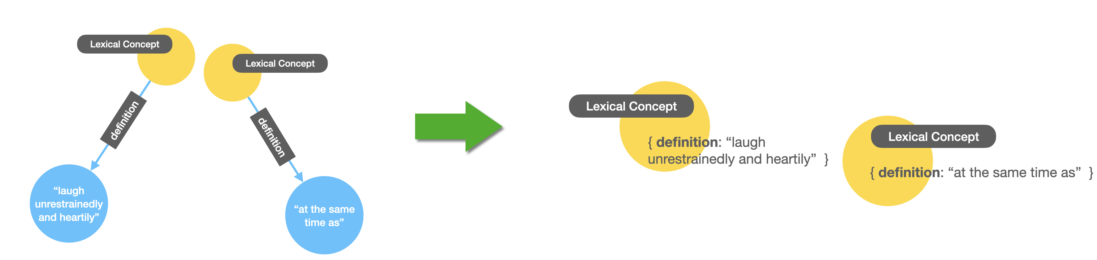
Every lexical concept has one and only one definition, represented in the RDF graph as a separate node with a single literal property containing the text representation of this form. This is not a very practical way to do it and we can make it a lot more compact by transforming the definition into a property of the lexical concept node. Here’s what I mean visually:

And here’s the cypher that runs the refactoring on the graph:

MATCH (n:ontolex__LexicalConcept)-[:wn__definition]-(def)
with n, collect(distinct def.rdf__value) as definitions
SET n.wn__definition = definitions[0]

Every lexical entry has a unique canonical form, represented in the RDF graph as a separate node with a single literal property containing the text representation of this form. This is not a very practical way to do it (even in RDF it could have been made simpler) but in our case we’ll make this a lot more compact by transforming the canonical form into a property of the lexical entry node. Here’s what I mean visually:

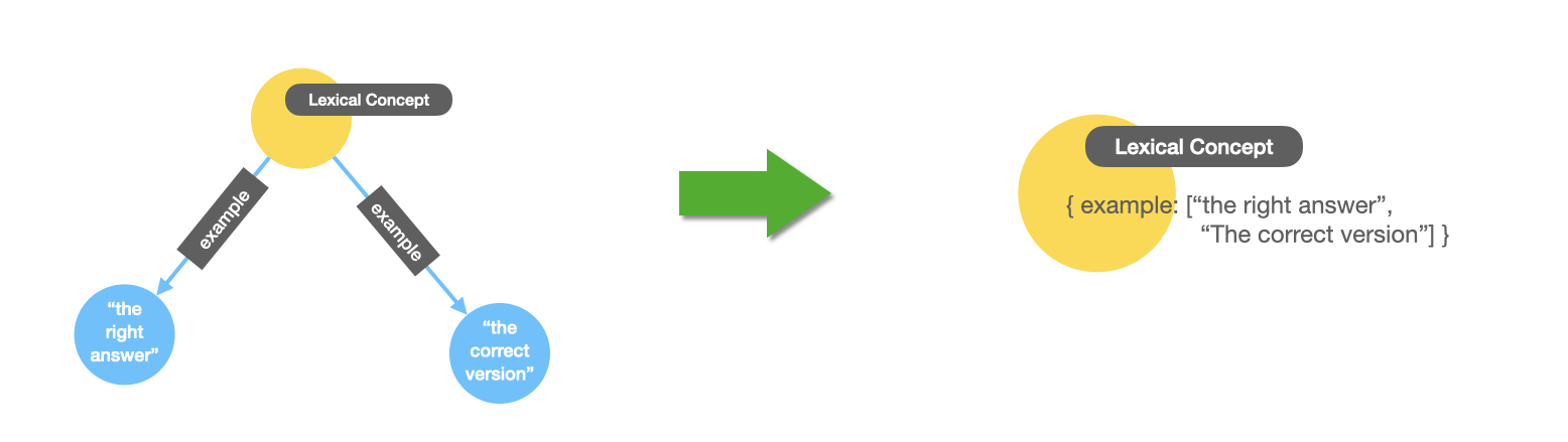
Multi-node to multivalued property refactoring: examples

A small variant of the previous pattern is the case of the examples for LexicalConcepts, we want to refactor them into properties of the LexicalConcepts like in the previous two cases, except that in this case there can be multiple values so we need to construct an array from it. Something like this:

And the cyhper:

MATCH (n:ontolex__LexicalConcept)-[:wn__example]->(ex) 
WHERE ex.rdf__value starts with "\"" and ex.rdf__value ends with "\""
WITH n, collect(distinct substring(ex.rdf__value, 1, size(ex.rdf__value)-2)) as examples
SET n.wn__example = examples ;

Node Deduplication and node to property refactoring: Canonical forms

Every lexical entry has one and only one canonical form, represented in the RDF graph as a separate node with a single literal property containing the text representation of this form. It is possible though that more than one lexical entry share the same canonical form. For instance break as a verb and break as a noun. In the RDF dataset these are represented by two different nodes which is not really useful, it would better if we could make it obvious the fact that they share the same canonical form by making them both connected to the same node representing this canonical form. We will do two things here. We’ll transform the canonical form into a property of the Lexical Entry and we will also keep the node representation but we will merge identical forms into one single node. Here’s what I mean visually:

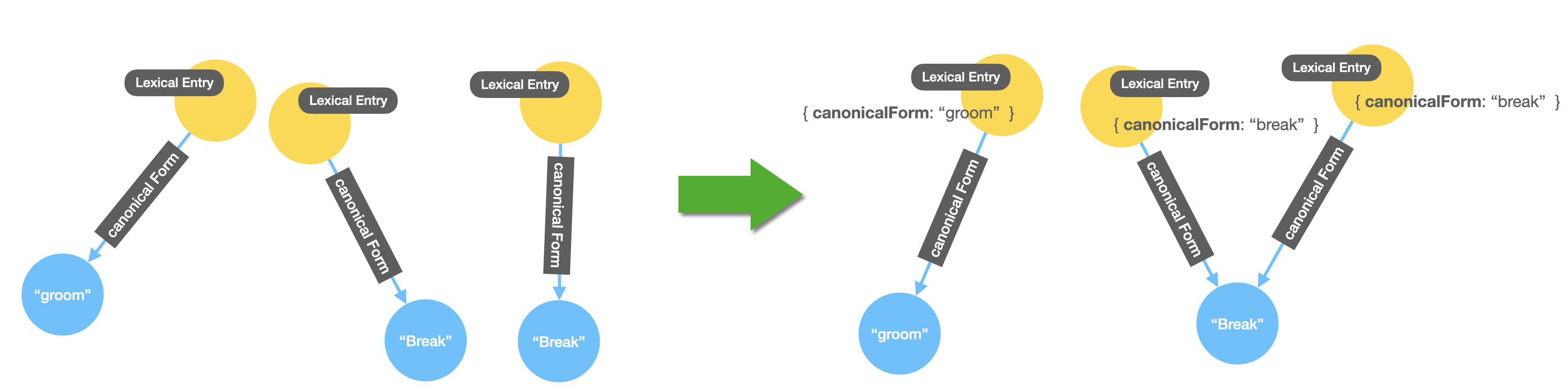
This refactoring step includes the previous node-to-property refactoring we saw before but it adds the refactoring step. You might be thinking why are we adding redundant information in the model by representing the canonical form in two different ways, both as a property and as a separate node. Well, you’re right, it is redundant but in some cases it can be beneficial from the point of view of performance or readability of the queries that you’ll write on the model. One thing you’ll have to keep in mind if you decide to do this is that you’ll have to be consistent later on when updating your model because if you update one of the representations and not the other (let’s say you update the property but not the node) you’ll find yourself with an inconsistent model that returns different results depending on how you query it. That said, it is not much of a problem in the case of the WordNet graph because the data is static.

Here’s the cypher that does the job. Notice that we do it in three steps. First we copy the existing values of the canonical form as properties of the lexical entry, then we remove the node representation and finally we recreate it, but this time making sure we introduce no duplicates (the MERGE keyword in cypher helps us with that).

//STEP 1
MATCH (n:ontolex__LexicalEntry)-[:ontolex__canonicalForm]-(cf)
with n, collect(distinct cf.ontolex__writtenRep) as canonicals
SET n.ontolex__canonicalForm = canonicals[0] ;

//STEP 2
MATCH (:ontolex__LexicalEntry)-[rel:ontolex__canonicalForm]-(cf)
DELETE rel, cf ;

//STEP 3
MATCH (le:ontolex__LexicalEntry)
MERGE (f:Resource { uri: apoc.text.replace(le.uri,"^(.*)#.*$","$1")}) 
    ON CREATE SET f.ontolex__writtenRep = le.ontolex__canonicalForm, f:ontolex__Form 
MERGE (le)-[:ontolex__canonicalForm]->(f) ;

The English WordNet Graph in Neo4j

So what does the resulting graph look like? Well, you can have a look yourself in this demo instance that we have published for you. Use the following credentials user:wordnet / pwd:wordnet.

The main structure of the graph is as follows: LexicalEntries are connected to one or many LexicalSenses through the sense relationship, and LexicalSenses have one and only one LexicalConcept associated. The last two are linked through the is lexicalized sense relationship. Here’s what it looks visually:

And here is a fragment of the graph where we can see how multiple Lexical senses converge on the same Lexical Concept, and similarly different senses for the same entry connect it to different Concepts:

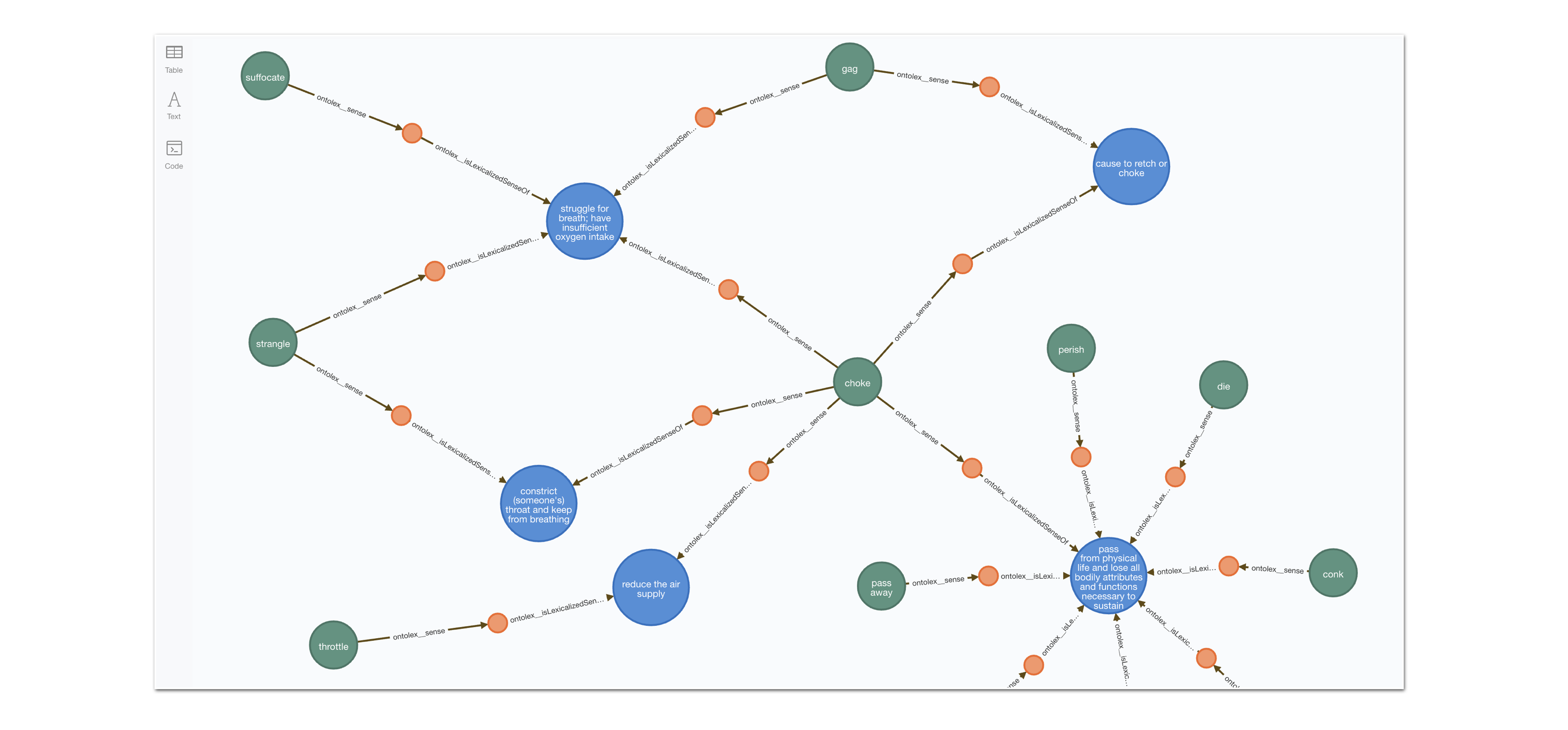
This cypher fragment will get you the previous graph excerpt:

MATCH path = (n:ontolex__LexicalEntry)-[:ontolex__sense]->()-[:ontolex__isLexicalizedSenseOf]->()<-[:ontolex__isLexicalizedSenseOf]-()<-[:ontolex__sense]-() 
RETURN path LIMIT 25

Lexical Concepts are also interconnected through different types of relationships such as synonymy, hypernymy, antonymy and meronymy among others. The following screen capture shows how chains of hypernym relationships form taxonomies of LexicalConcepts.

You can get the previous fragment or a similar one with the following query:

MATCH path = (n:ontolex__LexicalConcept)-[:wn__hypernym*..3]->(:ontolex__LexicalConcept) 
RETURN path LIMIT 25

What’s interesting about this QuickGraph?

As usual, the ease of construction is one of the things that will definitely surprise you. I hope you’ll find interesting and useful the refactoring steps that I went though because they can be useful in many contexts.

We will prove in the next QuickGraph that the extra refactoring effort pays off when writing sophisticated queries and analysis on the dataset.

One interesting aspect that we have not touched on in this QG but that we will definitely explore in the next is that you still can publish the English WordNet graph or parts of it as RDF from Neo4j should your consumer applications prefer it in this serialisation format.

See you next week in the second part of this QuickGraph and as always get the latest releases of Neo4j and n10s, and give it a go yourself! When you’re done, share your experience or your questions on the neo4j community site.