QuickGraph#10 Enrich your Neo4j Knowledge Graph by querying Wikidata

Wikidata is a collaboratively edited knowledge base. It is a source of open data that you may want to use in your projects. Wikidata offers a query service for integrations. In this QuickGraph, I will show how to use the Wikidata Query Service to get data into Neo4j.

The data source

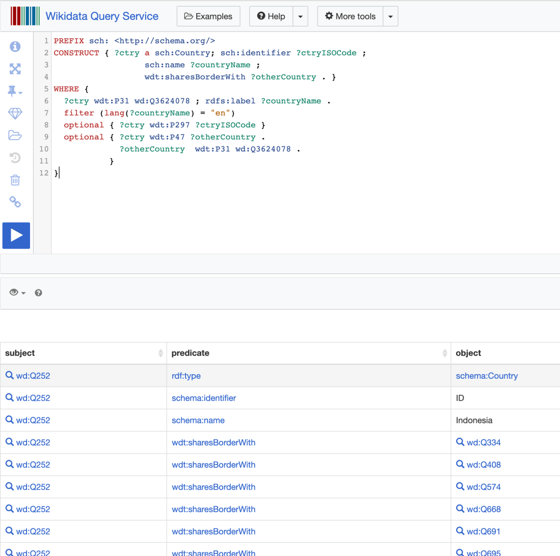
The Wikidata Query Service uses the SPARQL query language. For the first example in this QuickGraph, I will use a simple query that returns all countries in the world and for each of them, information on its neighbouring countries. This is the query:

PREFIX sch: <http://schema.org/> 
CONSTRUCT { ?ctry a sch:Country; sch:identifier ?ctryISOCode ; 
                  sch:name ?countryName ;
                  wdt:sharesBorderWith ?otherCountry . }
WHERE {
  ?ctry wdt:P31 wd:Q3624078 ; rdfs:label ?countryName .
  filter (lang(?countryName) = "en")  
  optional { ?ctry wdt:P297 ?ctryISOCode } 
  optional { ?ctry wdt:P47 ?otherCountry .
             ?otherCountry  wdt:P31 wd:Q3624078 .
           }
}

The only tricky bit in it (assuming you are familiar with SPARQL, of course) is Wikidata’s terminology. You can find more about it in their documentation, but these are the terms used in the query:

• wdt:P31 is the ‘Instance Of’ relationship.
• wd:Q3624078 is the ‘Sovereign state’ category. A country.
• wdt:P297 is the ISO 3166-1 alpha-2 country code.
• wdt:P47 is the ‘shares border with’ relationship.

The SPARQL savvy readers will notice that in my query I am also translating the Wikidata statements into terms of the more human-readable schema.org vocabulary. More specifically, I am producing sch:identifier statements for each wdt:P297, and adding the sch:Country type to every country as well as naming them using sch:name.

You can test the query in the Wikidata Query Service UI and you will see the results returned as RDF triples (subject, predicate, object):

The UI is great to write your query and see the results it produces but when it comes to importing the data programmatically into Neo4j, we will want them serialised in any of the standard RDF formats. For this example, we will use JSON-LD.

In order to get the results as RDF we just need to send an HTTP GET request to https://query.wikidata.org/ with a single parameter called sparql containing the text of the query (URL encoded). We will also need to add an ‘Accept’ header parameter with value ‘application/ld+json’ for the service to produce the desired serialisation format (JSON-LD).

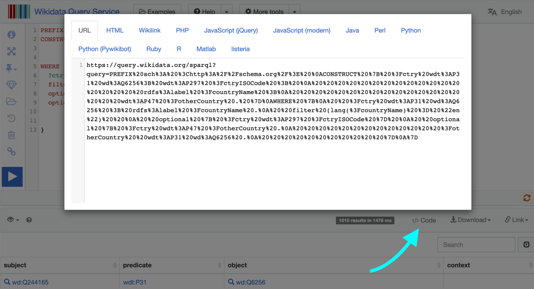
We can also test this. An easy way to get the full URL (including the encoded text of the query) is from the UI: on top of the results section, you will see a ‘code’ button that produces some code snippets showing how to use the query service with different programming languages. Take the first one (URL).

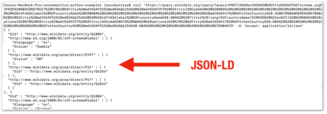
Now we can run this on a terminal:

curl 'https://query.wikidata.org/sparql?query=<...url encoded sparql...>' -H 'Accept: application/ld+json'

And if everything goes well we should see something like this:

Importing the data with Neosemantics

As we saw before, RDF represents information as statements, and statements form a graph which is something Neo4j is great at, so you’d think that import should be easy (and fully automated). You’re right! It is possible to load RDF easily into Neo4j using the Neosemantics plugin.  Here is how to do it from the Neo4j browser:

First, we define a Neo4j query parameter that we call sparql with the text of the SPARQL query as its value:

:PARAM sparql: 'PREFIX sch: <http://schema.org/> CONSTRUCT { ?ctry a sch:Country; sch:identifier ?ctryISOCode ; sch:name ?countryName ; wdt:sharesBorderWith ?otherCountry . } WHERE { ?ctry wdt:P31 wd:Q3624078 ; rdfs:label ?countryName . filter (lang(?countryName) = "en") optional { ?ctry wdt:P297 ?ctryISOCode } optional { ?ctry wdt:P47 ?otherCountry . ?otherCountry wdt:P31 wd:Q3624078 . } }'

Then we build the complete HTTP GET request by adding the URL of the query service and encoding the SPARQL query with APOC’s apoc.text.urlencode. We are also setting a header parameter with our choice of serialisation format.

CALL n10s.graphconfig.init( {handleVocabUris: "IGNORE"});

CALL n10s.rdf.import.fetch("https://query.wikidata.org/sparql?query=" + apoc.text.urlencode($sparql), "JSON-LD", { headerParams: { Accept: "application/ld+json"} });

Note that the serialisation produced by the Wikidata Query service needs to match the one set in the importRDF procedure:  We are using ‘application/ld+json’ in the headerParams of the request and “JSON-LD” in the format parameter of the importRDF procedure, but we could similarly use ‘application/rdf+xml’ and “RDF/XML” respectively and the effect would be identical.

Have a look at all the import parameters in the Neosemantics manual.

Exploring the data in Neo4j

Now we have the country dataset from Wikidata in Neo4j. We have nodes representing the countries and relationships representing border sharing between them. The first thing we notice is that even though the border sharing relationship is symmetrical, it is represented in both directions in Wikidata. Hence the double link between most nodes in the visual representation.

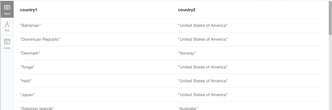
This is not a problem, but we could ‘clean’ this in our graph -or make it more LPG friendly– and keep a single relationship between two countries when they share a border. Also, as we will see in some of the following queries, Wikidata may have information gaps, for example, some borders present only on one side. We can write a query that identifies such cases.

MATCH (c:Country)-[:sharesBorderWith]->(neighbor)
WHERE NOT (neighbor)-[:sharesBorderWith]->(c)
RETURN c.name as country1, neighbor.name as country2

Which returns:

Path expressions

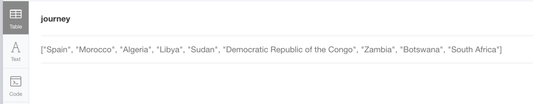
We can write simple path expressions like the following returning the shortest journey (as in ‘least number of borders crossed’) between Spain and South Africa:

MATCH sp = shortestPath((:Country { identifier: "ES"})-[:sharesBorderWith*]-(:Country { identifier: "ZA"}))
RETURN sp

This variant of the query returns the path as a sequence of node names instead:

MATCH sp = shortestPath((:Country { identifier: "ES"})-[:sharesBorderWith*]-(:Country { identifier: "ZA"}))
RETURN [c in nodes(sp) | c.name ] AS journey

Graph Algorithms

Warning: The Graph Algorithms library has been deprecated, so the code in this section may not be valid anymore. Please see the Graph Data Science (GDS) docs.

We can run some algos from the Neo4j Graph Algorithm Library on our dataset. Here’s an example of a simple centrality analysis:

CALL algo.betweenness.stream('Country','sharesBorderWith',{direction:'both'})
YIELD nodeId, centrality
MATCH (c:Country) WHERE id(c) = nodeId
WITH c, size((c)--()) AS degree, centrality WHERE degree > 0
RETURN c.name AS country, c.identifier AS code, degree, centrality, centrality/degree AS metric
ORDER BY metric DESC

This Cypher fragment runs a betweenness centrality computation on our graph and then weighing the results by bringing in the degree of each country (how many direct neighbours it has) to emphasise the centrality of weakly connected nodes (take this experiment as me showing how existing algorithms can be tuned to specific needs rather than a well-thought variant of the betweenness algorithm). Here are the results that it produces:

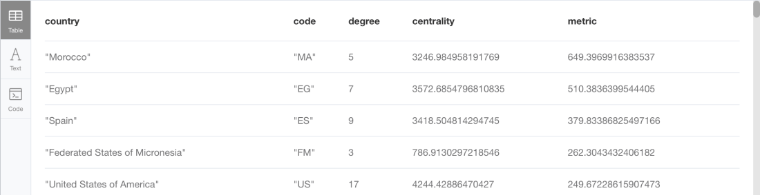
Countries like Morocco (MA), Egypt (EG) or Spain (ES), with a medium betweenness centrality score, are boosted because they have a relatively low degree.

Visual exploration insights

Probably the most beautiful outcome of this QuickGraph has been this diagrammatic map of the continents based only on the sharesBorderWith relationships in the graph. I have just added the blocks representing the continents behind the nodes in the browser but you can REALLY see them, right? I found this really cool. You can see the Mediterranean in the graph, right? The Indian Ocean.. even the Black sea and the Caspian sea are this gap in the centre!

To make it more intuitive I have marked some significant nodes: some connecting continents like Morocco linking Africa to Europe via Spain, or Russia sitting between Europe and Asia. Also some of the more highly connected ones: China, Indonesia, DRC or USA.

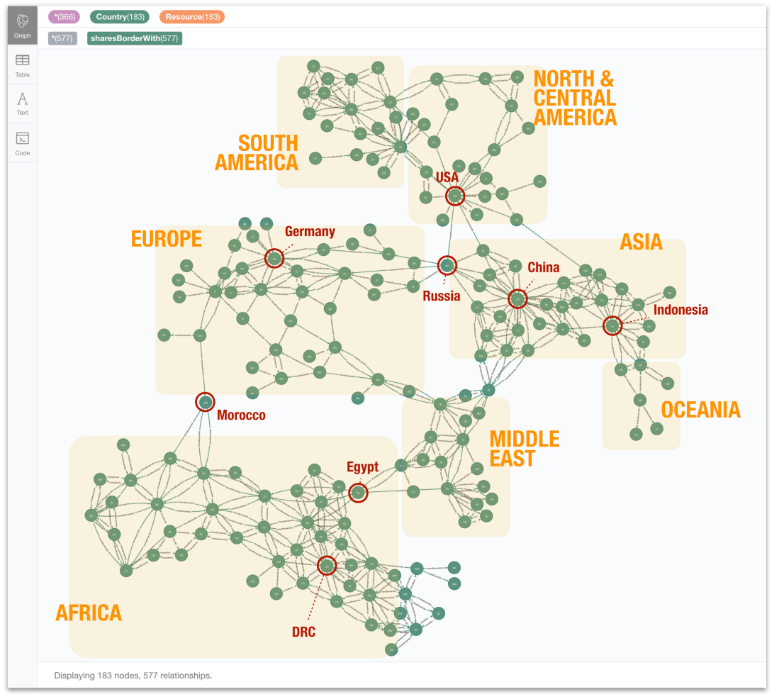
There are also some anomalies, like the UK and Ireland hanging off South America (!!). This is caused by the UK sharing a border with Venezuela. Maybe the pre-1966 British Guyana? Or maybe there is some current maritime border between the West Indies and Venezuela? No idea, but does not really matter for my QuickGraph, just a fun fact in the visualisation.

Dynamically extend the Knowledge Graph

Let’s say we want to enrich our country graph by representing the continents and linking the country nodes to the continent they are part of. The following SPARQL query returns the continent information for a given country. Notice the <…country URI…> placeholder where we will inline the country’s URI.

PREFIX sch: <http://schema.org/> 
CONSTRUCT { ?continent a sch:Continent ; sch:containsPlace ?ctry ; 
               rdfs:label ?continentName  }
WHERE {
  ?ctry wdt:P30 ?continent .
  filter(?ctry = <...country URI...>)
  ?continent rdfs:label ?continentName .
  filter (lang(?continentName) = "en")    
}

The only Wikidata term used in this query is wdt:P30 , the ‘continent’ relationship, which again, I am translating into a more humane from the schema.org vocabulary. I will use sch:containsPlace which is the generic containment relationship for Places.

This cypher fragment that does the job:

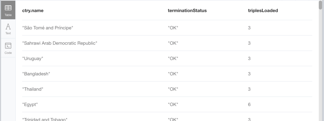
MATCH (ctry:Country) WITH 'PREFIX sch: <http://schema.org/> CONSTRUCT { ?continent a sch:Continent ; sch:containsPlace ?ctry ; rdfs:label ?continentName } WHERE { ?ctry wdt:P30 ?continent . filter(?ctry = <' + ctry.uri +'>) ?continent rdfs:label ?continentName . filter (lang(?continentName) = "en") }' AS continent_sparql, ctry CALL n10s.rdf.import.fetch("https://query.wikidata.org/sparql?query=" + apoc.text.urlencode(continent_sparql),"JSON-LD", { headerParams: { Accept: "application/ld+json"} , handleVocabUris: "IGNORE"}) YIELD terminationStatus, triplesLoaded RETURN ctry.name, terminationStatus, triplesLoaded

For every country found in the graph (ctry:Country), a request is sent to Wikidata to retrieve the continent information which is then imported into the graph via CALL n10s.rdf.import.fetch(…  The result shows the termination status for each country/request and the number of RDF triples imported.

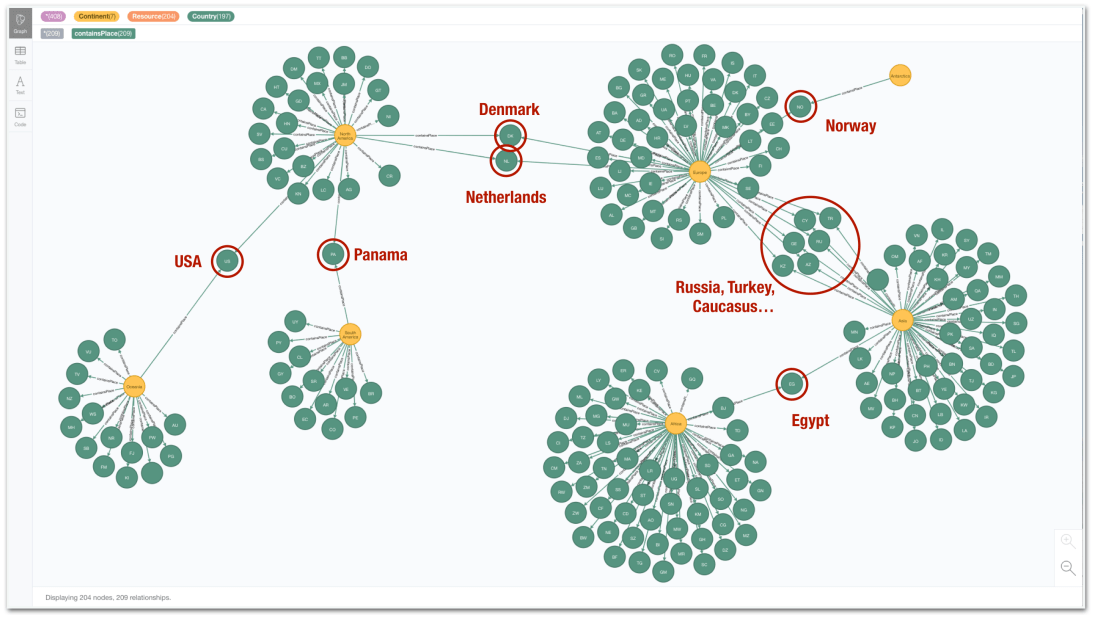
The resulting graph now includes nodes representing the continents, connected to the countries through the containsPlace relationship. A visualisation of these relationship reveals the cross-continent countries like Egypt, Turkey or Russia but shows also some (surprising?) results like the Netherlands, appearing both in Europe and in North America because of Suriname, one of its territories in America, and similarly Denmark because of Greenland. The same happens with the US (both in American and Oceania) probably because of Hawaii?

Again the data is probably not perfect but the point of this QuickGraph was not to run revealing analytics but to show how to create simple integrations to dynamically get Wikidata fragments into Neo4j.

What’s interesting about this QuickGraph?

We’ve shown how we can leverage existing data services producing RDF data to enrich our Knowledge Graph in Neo4j.  Because RDF is a graph, the Neosemantics plugin can ingest it without having to write much code. And speaking of code, the cypher used in this QuickGraph is, as usual, available in GithHub.

Give it a try and share your experience!