The scenario

Retail banking: Your graph-based fraud detection system powered by Neo4j is being used as part of the controls run when processing line of credit applications or when accounts are provisioned. It’s job is to block -or at least to flag- potentially fraudulent submissions as they come into your systems. It’s also sending alarms to fraud operations analysts whenever unusual patterns are detected in the graph so they can be individually investigated ASAP.

This is all working great but you want other analysts in your organisation to benefit from the super rich insights that your graph database can deliver, people whose job is not to react on the spot to individual fraud threats but rather understand the bigger picture. They are probably more strategic business analysts, maybe some data scientists doing predictive analysis too and they will typically want to look at fraud patterns globally rather than individually, combine the information in your fraud detection graph with other datasources (external to the graph) for reporting purposes, to get new insights, or even to ‘learn’ new patterns by running algorithms or applying ML techniques.

In this post I’ll describe through an example how Data Virtualization can be used to integrate your Neo4j graph with other data sources providing a single unified view easy to consume by standard analytical/BI tools.

Don’t get confused by the name, DV is about data integration, nothing to do with hardware  or infrastructure virtualization.

The objective

I thought a good example for this scenario could be the creation of an integrated dashboard on your fraud detection platform aggregating data from a couple of different sources.

Nine out of ten times integration will be synonym of ETL-ing your data into a centralised store or data warehouse and then running your analytics/BI from there. Fine. This is of course a valid approach but it also has its shortcomings, specially regarding agility, time to solution and cost of evolution just to name a few. And as I said in the intro, I wanted to explore an alternative approach, more modern and agile, called data virtualization or as it’s called these days, I’ll be building a logical data warehouse.

The “logical” in the name comes from the fact that data is not necessarily replicated (materialised) into a store but rather “wrapped” logically at the source and exposed as a set of virtual views that are run on demand. This is what makes this federated approach essentially different from the ETL based one.

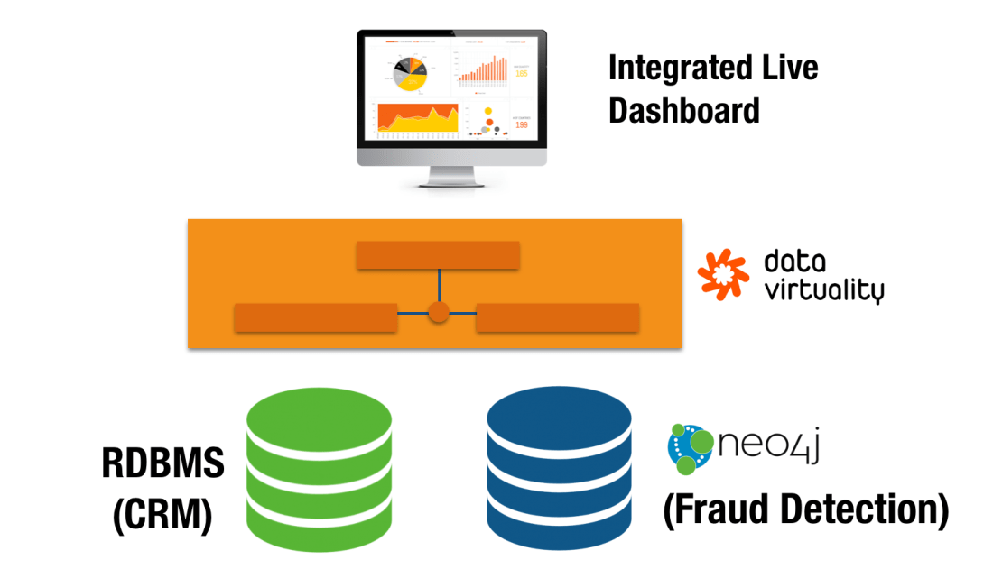
The architecture of my experiment is not too ambitious but rich enough to prove the point. It uses an off the shelf commercial data virtualization platform (Data Virtuality) abstracting and integrating two data sources (one relational, one graph) and offering a unified view to a BI tool.

Before I go into the details, a quick note of gratitude: When I decided to go ahead with this experiment, I reached out to Data Virtuality, and they very kindly gave me access to a VM with their data virtualization platform preinstalled and supported me along the way. So here is a big thank you to them, especially to Niklas Schmidtmer, a top solutions engineer who has been super helpful and answered all my technical questions on DV.

The data sources

 

Neo4j  for fraud detection

In this post I’m focusing on the integration aspects so I will not go into the details of what a graph-based fraud detection solution built on Neo4j looks like. I’ll just say that Neo4j is capable of keeping a real time view of your account holders’ information and detect potentially fraudulent patterns as they appear. By “real time” here, I mean as accounts are provisioned or updated in your system, or as transactions arrive, or in other words, as suspicious patterns are formed in your graph.

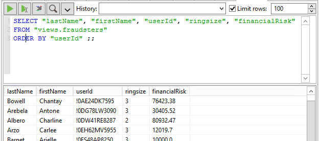
In our example, say we have a Cypher query returning the list of potential fraudsters. A potential fraudster in our example is an individual account holder involved in a suspicious ring pattern like the one in the Neo4j browser capture below. The query also returns some additional information derived from the graph like the size of the fraud ring and the financial risk associated with it. The list of fraudsters returned by this query will be driving my dashboard but we will want to enrich them first with some additional information from the CRM.

For a detailed description of what first party bank fraud is and how graph databases can fight it read this post.

 

RDBMS backed CRM system

The second data source is any CRM system backed by a relational database. You can put here the name of your preferred one or whichever in-house built solution your organisation is currently using.

The data in a CRM is less frequently updated and contains additional information about our account holders.

Data Virtualization

As I said before, data virtualization is a modern approach to data integration based on the idea of data on demand. A data virtualization platform wraps different types of data sources: relational, NoSQL, APIs, etc… and makes them all look like relational views. These views can then be combined through standard relational algebra operations to produce rich derived (integrated) views that will ultimately be consumed by all sorts of BI, analytics and reporting tools or environments as if they came from a single relational database.

The process of creating a virtual integrated view of a number of data sources can be broken down in three parts. 1) Connecting to the sources and virtualizing the relevant elements in them to create base views, 2) Combining the base views to create richer derived ones and 3) publishing them for consumption by analytical and BI applications. Let’s describe each step in a bit more detail.

Connecting to the sources from the data virtualization layer and creating base views

The easiest way to interact with your Neo4j instance from a data virtualization platform is through the JDBC driver. The connection string and authentication details is pretty much all that’s needed as we can see in the following screen capture.

Once the data source is created, we can easily define a virtual view on it based on our Cypher query with the standard CREATE VIEW… expression in SQL. Notice the usage of the ARRAYTABLE function to take the array structure returned by the request and produce a tabular output.

Once our fraudsters view is created, it can be queried just as if it was a relational one. The data virtualization layer will take care of the “translation” because obviously Neo4j actually talks Cypher and not SQL.

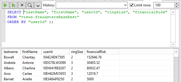
If for whatever reason you want to hit directly Neo4j’s HTTP REST API, you can do that by creating a POST request on the Cypher transactional endpoint and building the JSON message containing the Cypher (find description in Neo4j’s developer manual here). In Data Virtuality this can easily be done through a web service data import wizard, see next screen capture:

You’ll need to provide the endpoint details, the type of messages exchanged, the structure of the request. The wizard will then send a test request to figure out what the returned structure looks like and offer you a visual point and click way to select which values are relevant to your view and even offer a preview of the results.

Similar to the previous JDBC based case, now we have a virtual relational view built on our Cypher query that can be queried through SQL. Again the DV platform takes care of translating it into a HTTP POST request behind the scenes…

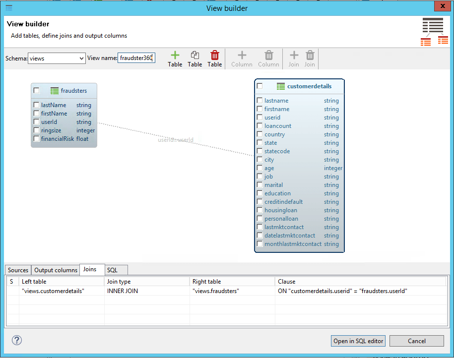
Now let’s go to the other data source, our CRM. Virtualizing relational datasources is pretty simple because they are already relational. So once we’ve configured the connection (identical to previous case, indicating server, port, and authentication credentials) the DV layer can introspect the relational schema and do the work for us by offering the tables and views discovered.

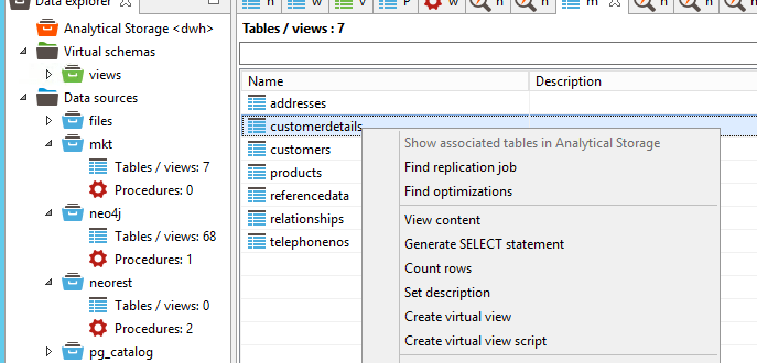
So we create a view on customer details from the CRM. This view includes the global user ID that we will use to combine this table with the fraudster data coming from Neo4j.

Combining the data from the two sources

Since we now hav two virtual relational views in our data virtualization layer, all we need to do is to combine them using a straightforward SQL JOIN. This can be achieved visually:

…or directly typing the SQL script

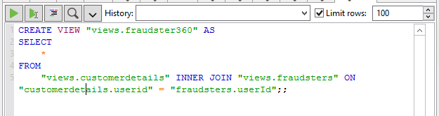
The result is a new fraudster360 view combining information from both our CRM system and the Neo4j powered fraud detection platform. As in the previous cases, it is a relational view that can be queried and most interestingly exposed to consumer applications.

Important to note: no data movement at this point, data stays at the source. We are only defining a virtual view (metadata if you want). Data will be retrieved on demand when a consumer application queries the virtual view as we’ll see in the next section.

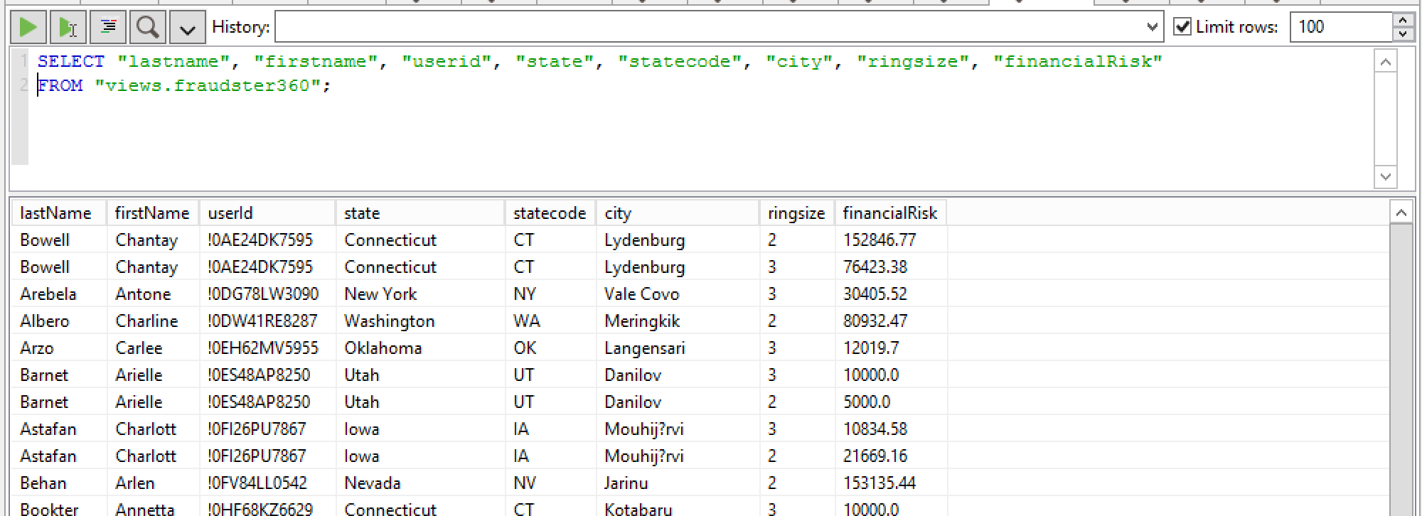
We can however test what will happen by running a test query from the Data Virtuality SQL editor. It is a simple projection on the fraudster360 view.

We can visualise the query execution plan to see that…

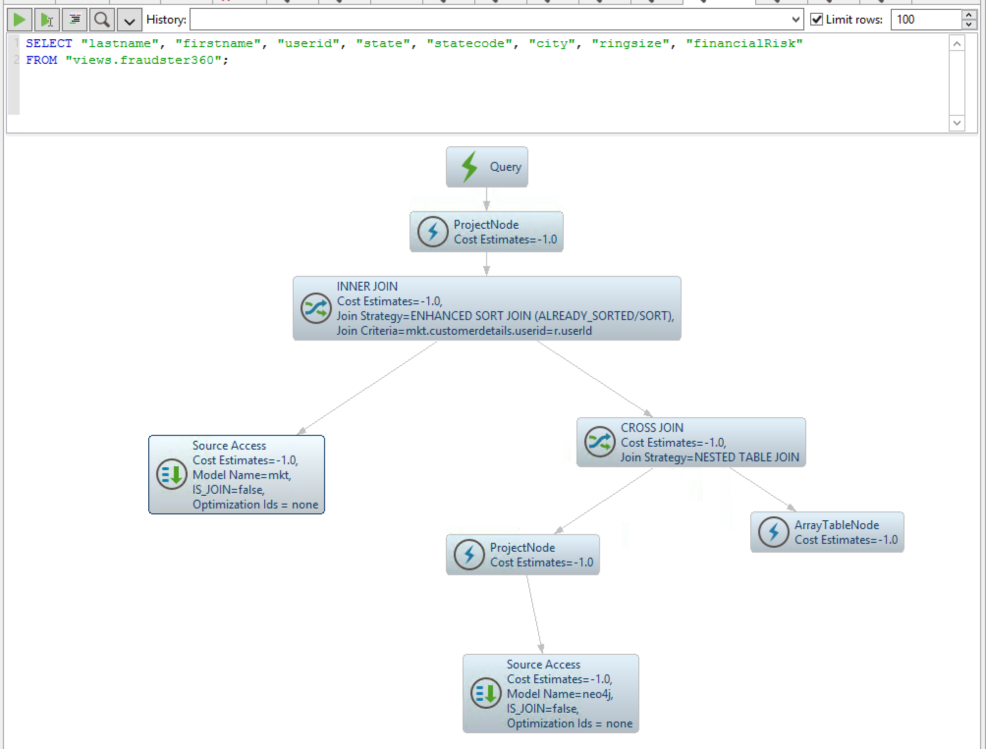
…the query on the fraudster360 is broken down into two, one hitting Neo4j and the other the relational DB. The join is carried out on the fly and the results streamed to the requester.

Even though I’m quite familiar with the data virtualization world, it was not my intention in this post to dive too deep into the capabilities of these platforms. Probably worth mentioning though that it is possible to use the DV layer as a way to control access to your data in a centralised way by defining role based access rules. Or that DV platforms are pretty good at coming up with execution plans that delegate down to the sources as much of the processing as possible, or alternatively, caching a the virtual level if the desired behavior is precisely the opposite (i.e. protecting the sources from being hit by analytical/BI workload).

But there is a lot more, so if you’re interested, ask the experts.

Exposing composite views

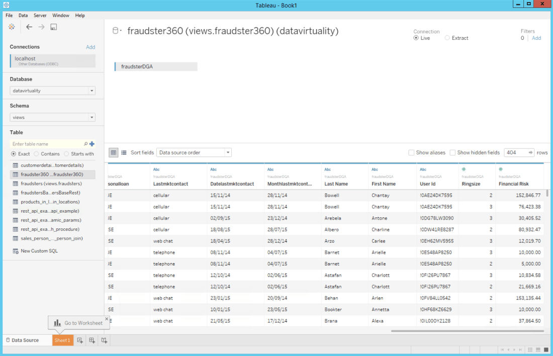
I’ll use Tableau for this example. Tableau can connect to the Data Virtualization server via ODBC. The virtual views created in Data Virtuality are listed and all that needs to be done is selecting our fraudster360 view and check that data types are imported correctly.

I’m obviously not a Tableau expert but I managed to easily create a couple of charts and put them into a reasonably nice looking dashboard. You can see it below, it actually shows how the different potential fraud cases are distributed by state, how does the size of a ring (group of fraudsters collaborating) relate to the financial risk associated with it or how these two factors are distributed regionally.

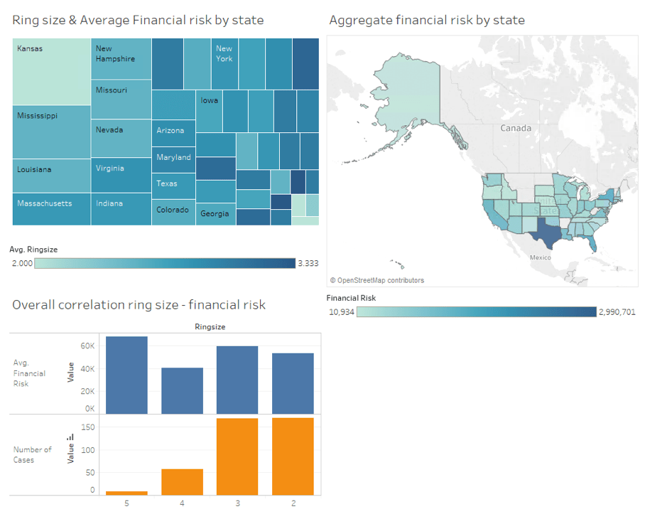
And the most interesting thing about this dashboard is that since it is built on a virtual (non materialised) view, whenever the dashboard is re-opened or refreshed, the Data Virtualization layer will query the underlying Neo4j graph for the most recent fraud rings and join them with the CRM data so that the dashboard is guaranteed to be built on the freshest version of data from both all sources.

Needless to say that if instead of Tableau you are a Qlik or an Excel user, or you write R or python code for data analysis, you would be able to consume the virtual view in exactly the same way (or very similar if you use JDBC instead of ODBC).

Well, that’s it for this first experiment. I hope you found it interesting.

Takeaways

Abstraction: Data virtualization is a very interesting way of exposing Cypher based dynamic views on your Neo4j graph database to non technical users making it possible for them to take advantage of the value in the graph without necessarily having to write the queries themselves. They will consume the rich data in your graph DB through the standard BI products they feel comfortable with (Tableau, Excel, Qlik, etc).

Integration: The graph DB is a key piece in your data architecture but it will not hold all the information and integration will be required sooner or later. Data Virtualization proves to be a quite nice agile approach to integrating your graph with other data sources offering controlled virtual integrated datasets to business users enabling self service BI.

Interested in more ways in which Data Virtualization can integrate with Neo4j? Watch this space.