QuickGraph#18 Semantic similarity metrics in taxonomies: A wikipedia example on uncrewed spacecraft

In this post i’ll give you an overview of some similarity metrics I’ve discovered when working with WordNet. Even though they were originally proposed as linguistic similarity metrics, I thought it would make sense to explore their behaviour if we generalise their use to a taxonomy-annotated dataset.

I will use public data from Wikipedia and what topic to choose on the week that Percy landed in Mars? No other than the rich domain of uncrewed spacecraft. Follow me!

Loading the Taxonomy in Neo4j

I’ll follow the process described in QG#6. We build the taxonomy by querying the MediaWiki API and processing the returned JSON with APOC. The code I wrote then still works nicely so I’ll just reuse it. I’ll copy it here for convenience. The approach is quite simple, we first create the root category: “Uncrewed_spacecraft” and then we iteratively add child categories until we reach the end of the taxonomy (the API returns no more results). Here are the details:

Let’s start by creating a few indexes to accelerate the ingestion and querying of the data:

CREATE INDEX ON :Category(catId);
CREATE INDEX ON :Category(catName);
CREATE INDEX ON :Page(pageTitle);

Now let’s create the root category. As we said before, we’ll use “Uncrewed_spacecraft”.

CREATE (c:Category:RootCategory {catId: 0, catName: 'Uncrewed_spacecraft', subcatsFetched : false, pagesFetched : false, level: 0 })

Next, we load the next level of subcategories iteratively. We will be running this step several times so I’ve defined a parameter with the level at which it works. So set the parameter before running it. We will start from the root category (level = 0) so we need to run :param level => 0 in the browser or the equivalent syntax in your language of choice if you’re doing this programatically using the drivers.

MATCH (c:Category { subcatsFetched: false, level: $level})
CALL apoc.load.json('https://en.wikipedia.org/w/api.php?format=json&action=query&list=categorymembers&cmtype=subcat&cmtitle=Category:' + apoc.text.urlencode(c.catName) + '&cmprop=ids%7Ctitle&cmlimit=500')
YIELD value as results
UNWIND results.query.categorymembers AS subcat
MERGE (sc:Category {catId: subcat.pageid})
ON CREATE SET sc.catName = substring(subcat.title,9),
 sc.uri ='https://en.wikipedia.org/wiki/Category:'+replace(subcat.title,' ', '_'),
 sc.subcatsFetched = false,
 sc.pagesFetched = false,
 sc.level = $level + 1
WITH sc,c
MERGE (sc)-[:SUBCAT_OF]->(c)
WITH DISTINCT c
SET c.subcatsFetched = true

That’s it. All you’ll need to do is iterate as many times as you want. Just set the param to the next value :param level => 1 and re-run the previous query. For this simple example it’s not a problem to do it manually since the taxonomy is not more than 7 or 8 levels deep but feel free to script the whole process.

Keeping the taxonomy tidy

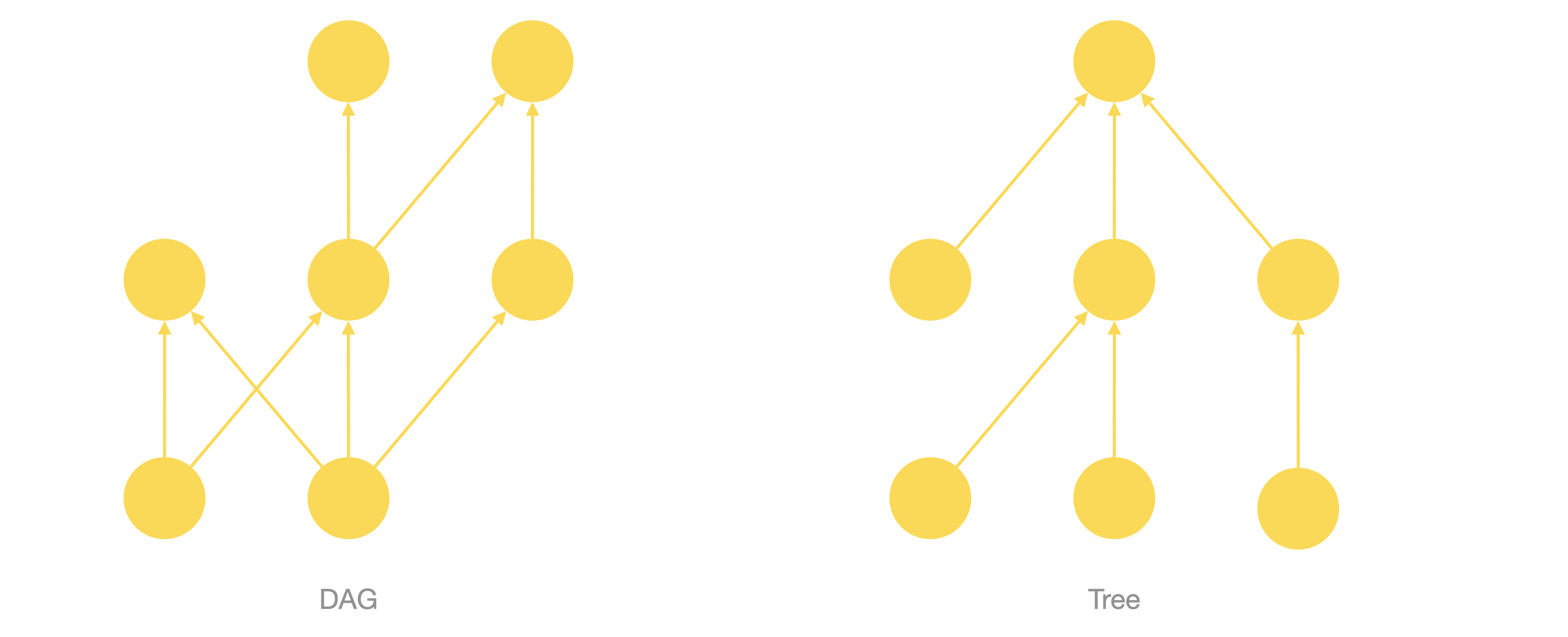
You will notice two things as you import the Wikipedia taxonomy: The first one is that it’s not a tree but a directed acyclic graph (DAG). This in other words means that any category can have multiple parent categories and not only one. This is what a DAG looks like compared to a tree.

The fact that it’s a DAG and not a tree is not a problem at all and is a pretty natural thing in collaboratively built taxonomies. An example of this situation would be the category “Cancelled NASA space probes” which is a subcategory both of “NASA space probes” and “Cancelled space probes“.

The second thing that you’ll notice is that sometimes there are redundant SUBCATEGORY_OF relationships, where a category is connected to its immediate super-category, but also to some other ancestor like in the diagram below. These can be problematic when we look at distance based similarity between categories, so wee will want to remove them as we see in the diagram below.

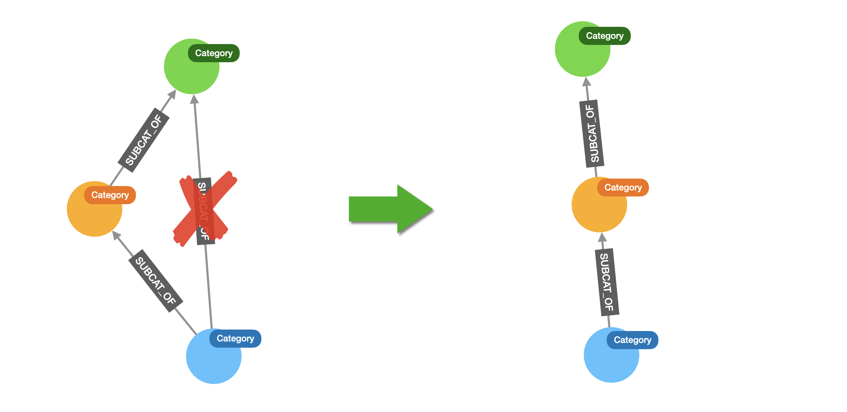
And there is a simple cypher query that will do the job for us:

MATCH (a)<-[shortcut:SUBCAT_OF]-(:Category)-[:SUBCAT_OF*2..]->(a)
DELETE shortcut

Adding the instances (the wikipedia pages)

Finally we can add the wikipedia pages to our model. We can think of them as the individuals or instances that are classified in the taxonomy. Here’s the cypher query that loads the pages:

MATCH (c:Category { pagesFetched: false })
CALL apoc.load.json('https://en.wikipedia.org/w/api.php?format=json&action=query&list=categorymembers&cmtype=page&cmtitle=Category:' + apoc.text.urlencode(c.catName) + '&cmprop=ids%7Ctitle&cmlimit=500')
YIELD value as results
UNWIND results.query.categorymembers AS page
MERGE (p:Page {pageId: page.pageid})
ON CREATE SET p.pageTitle = page.title, p.uri = 'http://en.wikipedia.org/wiki/' + apoc.text.urlencode(replace(page.title, ' ', '_'))
WITH p,c
MERGE (p)-[:IN_CATEGORY]->(c)
WITH DISTINCT c
SET c.pagesFetched = true

Sometimes (most of the times) a page will be connected to multiple categories. We find that a page can be connected to both a category C and a super-category of C creating redundant links like the one we described earlier. The following query will help removing these undesired redundancies.

MATCH (a:Category)<-[shortcut:IN_CATEGORY]-(page:Page)-[:IN_CATEGORY]->(cat)-[:SUBCAT_OF*1..]->(a)
DELETE shortcut

Exploring the taxonomy

Every wikipedia page will have at least one category and in the DAG, this category will be connected directly or indirectly to the root category: “Uncrewed_spacecraft“. Here is a simple query that shows us the page for the Perseverance probe and its full taxonomy:

MATCH tx = (p:Page)-[:IN_CATEGORY]->(:Category)-[:SUBCAT_OF*]->(:RootCategory)
WHERE p.pageTitle contains "Perseverance"
RETURN tx

producing the following result:

Semantic similarity metrics

Given two individuals (two wikipedia pages or categories in our case), the similarity metrics will compute a value (most of the times between 0 and 1 although not always as we will see) that indicates how closely related they are.

The first metric is the simplest and is purely based on graph distance.

Path similarity

This path similarity metric is based on the shortest path that connects the two elements in the taxonomy. This is how it is calculated:

It is easy to implement in plain cypher. Let’s test it comparing the similarity between the Mars rover Perseverance and the cargo spacecraft Kounotori 7 and that between the Kounotori 7 and the Albert Einstein transfer vehicle.

If we look at the first two, this pattern returns all the taxonomy paths between them.

:params { pageA: "Perseverance (rover)", pageB: "Kounotori 7"}

MATCH p = (a:Page { pageTitle: $pageA})-[:IN_CATEGORY]->(a_cat)-[:SUBCAT_OF*0..]->()<-[:SUBCAT_OF*0..]-(b_cat)<-[:IN_CATEGORY]-(b:Page { pageTitle: $pageB})
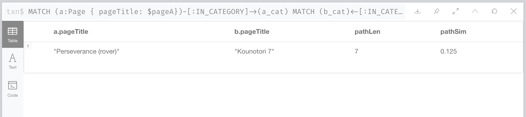
RETURN p

In the capture below, we can see that the shortest path between the Perseverance and the Kounotori is of lenght 7. One of the possible shortest paths is highlighted.

We can modify the previous query to return the path similarity metric as defined in the previous equation

MATCH (a:Page { pageTitle: $pageA})-[:IN_CATEGORY]->(a_cat)
MATCH (b_cat)<-[:IN_CATEGORY]-(b:Page { pageTitle: $pageB})
MATCH p = shortestPath((a_cat)-[:SUBCAT_OF*0..]-(b_cat))
WITH a, a_cat, b, b_cat, length(p) + 2  as pathLen
RETURN a.pageTitle, b.pageTitle, pathLen, 1.0/(1+pathLen) as pathSim
ORDER BY pathLen LIMIT 1

Producing the following result:

The same query applied to the pair Kounotori 7 and Albert Einstein cargo aircrafts, produce the following results:

:params { pageA: "Albert Einstein ATV", pageB: "Kounotori 7"}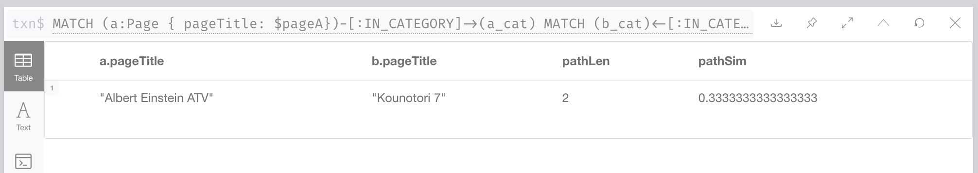

Even though it’s a basic one, the path similarity metric produces meaningful results and the two cargo aircrafts are three times closer (more similar) than either of them with the Perseverance Mars rover. But that said, it has some particularities that we may want to tune a little bit. One of them is that when comparing pages, the maximum similarity will be 0.33 when they are in the same category, and it will go down from there.

Also this metric is sensitive only to the path distance. Because of that, “shortcuts” in the taxonomy like the ones described earlier can make a big difference, and that’s why we removed them. But the fact that some branches of the taxonomy are more developed (more fine grained) than others will also have an important impact in this similarity metric because they will increase the distance between nodes and therefore reduce the similarity in a probably undesired way.

Leacock-Chodorow Similarity

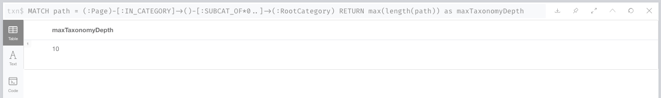
The Leacock-Chodorow similarity metric adds one additional element, and that is the depth of the taxonomy. We can easily compute the depth of a taxonomy as the greatest length of the path between any element and the root element. This is how we get depth of our taxonomy with Cypher:

MATCH path = (:Page)-[:IN_CATEGORY]->()-[:SUBCAT_OF*0..]->(:RootCategory)
RETURN max(length(path)) as maxTaxonomyDepth

Which in our case returns the following:

Note that in our example there is a single root category and that all categories are connected directly or indirectly to it but we could have scenarios where there are multiple root elements and therefore multiple sub-taxonomies. In those cases, we would need to compute the depth of the taxonomy containing the elements we are comparing.

The following equation shows how to calculate the Leacock-Chodorow similarity metric:

It essentially boosts similarities that happen in deeper hierarchies but since our example has a single taxonomy containing all elements, the results will be very similar to the ones we got from plain path similarity.

Let’s see what this looks like in cypher…

WITH 10 as taxonomyDepth //computed in previous step
MATCH (a:Page { pageTitle: $pageA})-[:IN_CATEGORY]->(a_cat)
MATCH (b_cat)<-[:IN_CATEGORY]-(b:Page { pageTitle: $pageB})
MATCH p = shortestPath((a_cat)-[:SUBCAT_OF*0..]-(b_cat))
WITH taxonomyDepth, a, a_cat, b, b_cat, length(p) + 2  as pathLen
RETURN a.pageTitle, b.pageTitle, pathLen, taxonomyDepth, -log10(pathLen * 1.0 / (2*taxonomyDepth))  as LCSim
ORDER BY pathLen LIMIT 1

and let’s see what it produces for the same pages we used before:

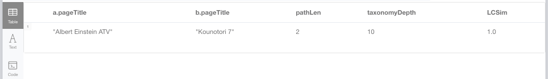
Interesting to notice that this metric can go over 1 if the ratio between the distance and the depth is smaller than 1/10.

Wu & Palmer similarity

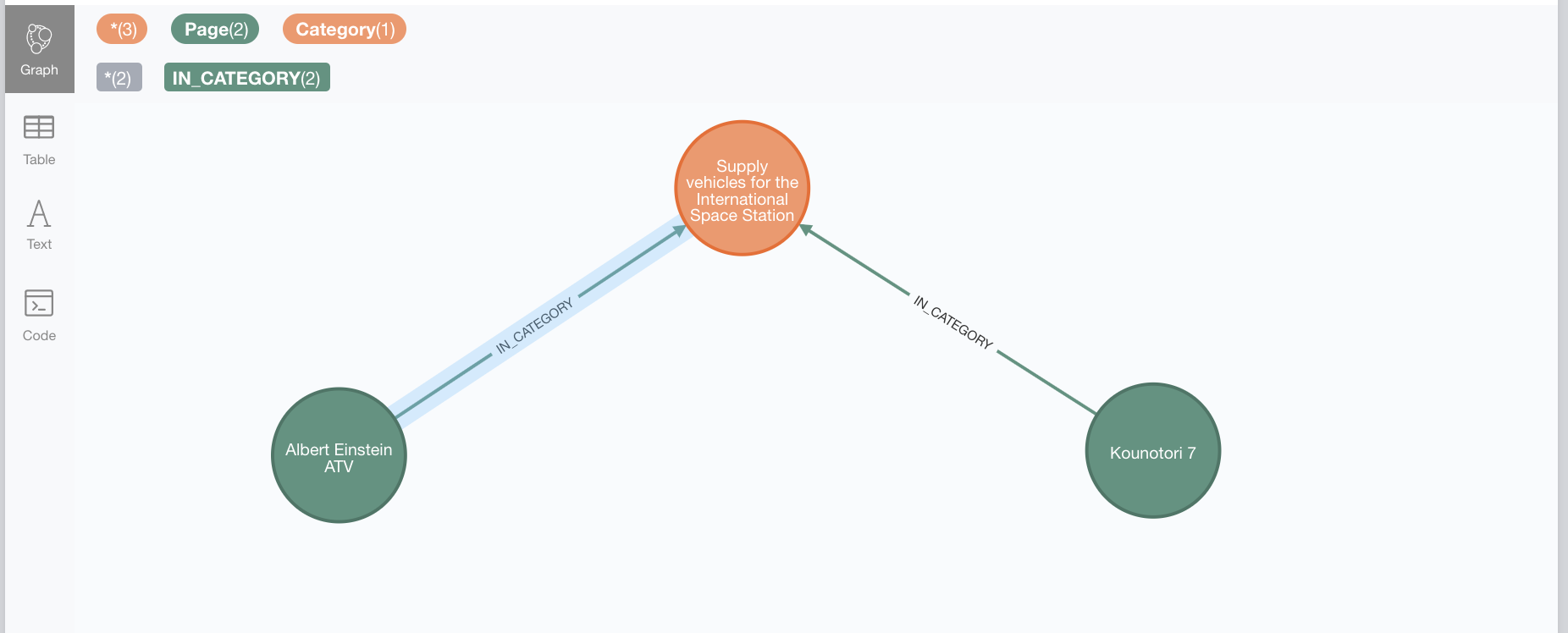
The Wu&Palmer similarity metric introduces one additional element, that of the Least Common Subsumer (LCS). The LCS is the most specific ancestor node of the two that are being compared. It is easy to get the LCS with cypher, we just need to draw the pattern as follows:

MATCH spa = (a:Page { pageTitle: $pageA })-[:IN_CATEGORY]->(a_cat) 
MATCH spb = (b:Page { pageTitle: $pageB })-[:IN_CATEGORY]->(b_cat) 
MATCH p = (a_cat)-[:SUBCAT_OF*0..]->(lcs)<-[:SUBCAT_OF*0..]-(b_cat) 
RETURN spa, spb, p 
ORDER BY length(p) LIMIT 1

Which would produce the following subgraph:

The Wu&Palmer similarity metric combines the depths of the two elements being compared and that of their LCS as follows:

And like we did before, we can encode this in a cypher expression:

MATCH (rc:RootCategory)
MATCH (a:Page { pageTitle: $pageA })-[:IN_CATEGORY]->(a_cat) 
MATCH (b:Page { pageTitle: $pageB })-[:IN_CATEGORY]->(b_cat) 
MATCH sp = (a_cat)-[:SUBCAT_OF*0..]->(lcs)<-[:SUBCAT_OF*0..]-(b_cat) 
WITH a, b, rc, a_cat, b_cat, lcs ORDER BY length(sp) LIMIT 1
WITH $pageA as pageA, $pageB as pageB, length(shortestPath((a)-[*]->(rc))) + 1 as depthA,
       length(shortestPath((b)-[*]->(rc))) + 1 as depthB, lcs.catName as LCS,
       length(shortestPath((lcs)-[*0..]->(rc))) +1 as depthLCS
RETURN pageA, depthA, pageB, depthB, LCS, depthLCS, 2.0 * depthLCS / (depthA + depthB) as WPSim

Which would return the following for the two cargo spacecraft

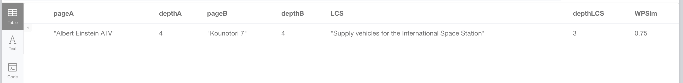
And for one of them and the Mars rover

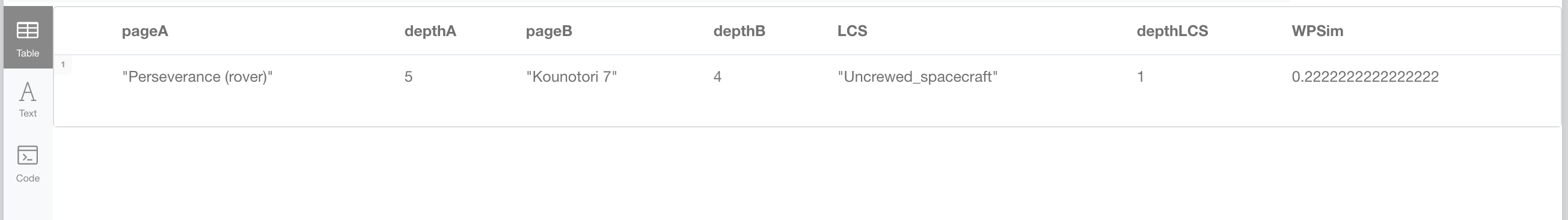
We can see that the depth of the LCS has a significant impact in this metric. For the Kounotori 7 and the Albert Einstein ATV, the LCS is the category “Supply vehicles for the international Space Station” (depth 3) while the LCS for the Kounotori 7 and the Perseverance is the root category: “Uncrewed spacecraft” (depth 1).

Also note that the WP similarity metric counts the depth of the root element as 1 hence the +1 added to the path length in the cypher fragment. This is to avoid the WP similarity metric to ever return 0.

Similarity metrics summary

The following table shows a summary of the similarity metrics we’ve described applied to a bunch of pages from the uncrewed aircraft wikipedia dataset compared to the Perseverance rover page.

I’ve highlighted in the previous table one case where the metrics differ significantly, that is the case of Perseverance vs Kepler-70c. Let’s analyse it.

First of all, you may ask yourself: hang on, how did an exoplanet like Kepler 70c end up in a taxonomy about uncrewed spacecraft? Well, the answer is that the wikipedia taxonomy is not a strict classification. You should think about it as a loose knowledge organisation system. The SUBCAT_OF relationships in our graph are closer to the broader/narrower than in SKOS than to the SubclassOf in RDFS. So basically SUBCAT_OF means that a concept is more general in meaning. With that context it’s probably easier to follow the visual explanation below:

So the Kepler 70c is an exoplanet that is tagged with the category “Exoplanets discovered by the Kepler space telescope”. You can see this from its wikipedia page (links to categories are at the bottom of the page). That category is itself under the “Kepler space telescope” which is under the “Discovery Program”, which is under “NASA space probes”… a couple more steps and you get to the root “Uncrewed spacecraft”. In addition to that, we can also see in the previous image that this is not the only path that connects the Kepler 70c to the root category.

Ok, so why if there’s a rather long path distance (distance 6) between the two elements do they become so “similar” according to the Wu Palmer metric? Well, it’s all about the depth of their LCS, which happens to be “NASA space probes”. Let’s overlay the taxonomies for both pages and highlight in it the shortest path. An image is worth a thousand words, so just watch it below:

Extra section: Publishing the taxonomy using SKOS

Although a bit tangential to the topic of the post, I thought not a bad idea to remind you that you can publish your graph (any graph that lives in a Neo4j database) as RDF with your vocabulary of choice.

I thought given the fact that ours contains a taxonomy, SKOS sounded like a good option so here’s what you’d need to do.

Map our model to the SKOS Vocabulary

Essentially we need to configure neo4j (via n10s) so that :Category(ies) in our model will be published as skos:Concept(s), that :SUBCAT_OF relationships will be published as skos:broader predicates and that category names in the catName properties are published as skos:prefLabel. Three pretty straightforward mappings. Here’s the code:

//add SKOS namespace and register prefix for it
CALL n10s.nsprefixes.add("skos","http://www.w3.org/2004/02/skos/core#");

//define mappings for Category, SUBCAT_OF and catName
CALL n10s.mapping.add("http://www.w3.org/2004/02/skos/core#Concept", "Category");
CALL n10s.mapping.add("http://www.w3.org/2004/02/skos/core#broader", "SUBCAT_OF");
CALL n10s.mapping.add("http://www.w3.org/2004/02/skos/core#prefLabel", "catName");

Query the Graph, get the RDF/SKOS

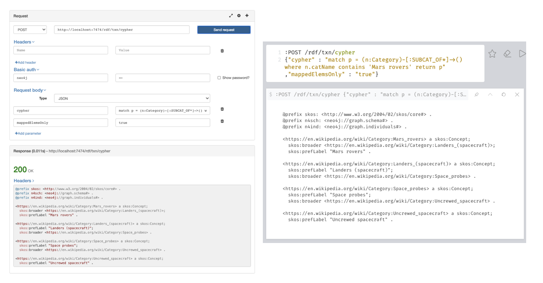
And you’re ready to go! Your RDF-consuming application can start querying the Neo4j RDF endpoint

You can test the many ways in which a Neo4j graph can be published as RDF directly in the browser using the :GET and :POST notation, or you can do it with any http client. I’ll use a chrome extension called RESTED and the browser to show what it looks like:

What’s interesting about this QuickGraph?

There are several great things about this #QG

• First, it shows one of the many ways in which a taxonomy-annotated dataset can be imported into Neo4j. In this case, we get it from the wikipedia rest endpoint producing easily consumable JSON.
• The #QG also gives an overview of three well-known similarity metrics taken from linguistic analysis and used in a generic taxonomy, explaining their internals from a graph point of view.
• I think the visual aspect of graphs was particularly helpful understanding how these metrics work, and eventually it can help us defining our own custom metrics or combining existing ones.

On the not so positive side, we see that “free” or “loose” taxonomies like the Wikipedia can show some unexpected/illogical behaviours like the one in the image below. A page is given multiple categories that are linked in a loose taxonomy that ultimately contradicts itself. It cannot really be considered a contradiction as in a logical inconsistency because the category taxonomy was never a formal logic theory but it can generate unexpected results and definitely complicates tasks like the one we covered in this post of computing similarities.

Thinking about it, this idea of finding contradictions in the wikipedia category structure could be an interesting topic for a future QuickGraph?

As always, give it a try using the instructions and queries in this post and share your experience or your questions on the neo4j community site.

Thanks for your interest, see you in the next QG.