- Applying transformations to the imported RDF graph to make it benefit from the LPG modelling capabilities and enriching the graph with additional complementary data sources.
- Querying the graph to do complex path analysis and use graph patterns to detect data quality issues like data duplication and also to profile your dataset
- Integrate Neo4j with standard BI tools to build nice charts on the output of Cypher queries on your graph.
- Building an RDF API on top of your Neo4j graph.
All the code I’ll use is available on GitHub. Enjoy!
The dataset
In this example, I’ll use the Open PermID dataset by Thomson Reuters. Here is a diagram representing the main entities we will find in it (from https://permid.org/).

I’ll be using for this experiment the dump from the 7th January 2018. You can download the current version of the dataset from the bulk download section. The data dump contains around 38 million triples 127million triples [Note: Halfway through the writing of this blog entry a new file containing person data was added to the downloads page increasing the size of the full dump by 300%. If you had looked at this dataset before, I recommend you have a look at the new stuff].
The Data import
The dump is broken down into 6 files named OpenPermID-bulk-XXX.ntriples (where XXX is Person, Organization, Instrument, Industry, Currency, AssetClass, Quote). I will import them into Neo4j as usual with the semantics.importRDF stored procedure that you can find in the neosemantics neo4j extension. I’ll use the N-Triples RDF serialization format but a Turtle one is also available.
Here is the script that will do the data load for you. You’ll find in it one call to the semantics.importRDF stored procedure per RDF file, just like this one:
CALL semantics.importRDF("file:////OpenPermID/OpenPermID-bulk-organization-20180107_070346.ntriples","N-Triples", {})
The data load took just over an hour on my 16Gb MacBook Pro and while this may sound like a modest load performance (~35K triples ingested per second), we have to keep in mind that in Neo4j all connections (relationships) between nodes are materialised at write time as opposed to triple stores or other non-native graphs stores where they are computed via joins at query time. So it’s a trade-off between write and read performance: with Neo4j you get more expensive transactional data load but lightning speed traversals at read time.
Also worth mentioning that the approach described here is transactional which may or may not be the best choice when loading super-large datasets. It’s ok for this example because the graph is relatively small for neo4j standards, but if your dataset is really massive you may want to consider alternatives like the non-transactional import tool (https://neo4j.com/docs/operations-manual/current/import/).
I completed the data load by importing the countryInfo.txt file from Geonames to enrich the country information that in the PermID data export is reduced to URIs. The Geonames data is tabular so I used the following LOAD CSV script:
LOAD CSV WITH HEADERS from "file:///OpenPermID/countryInfo.txt" as row fieldterminator '\t'
MATCH (r:Resource { uri: "http://sws.geonames.org/" + row.geonameid + "/" } )
SET r+= row, r:Country;
The imported graph
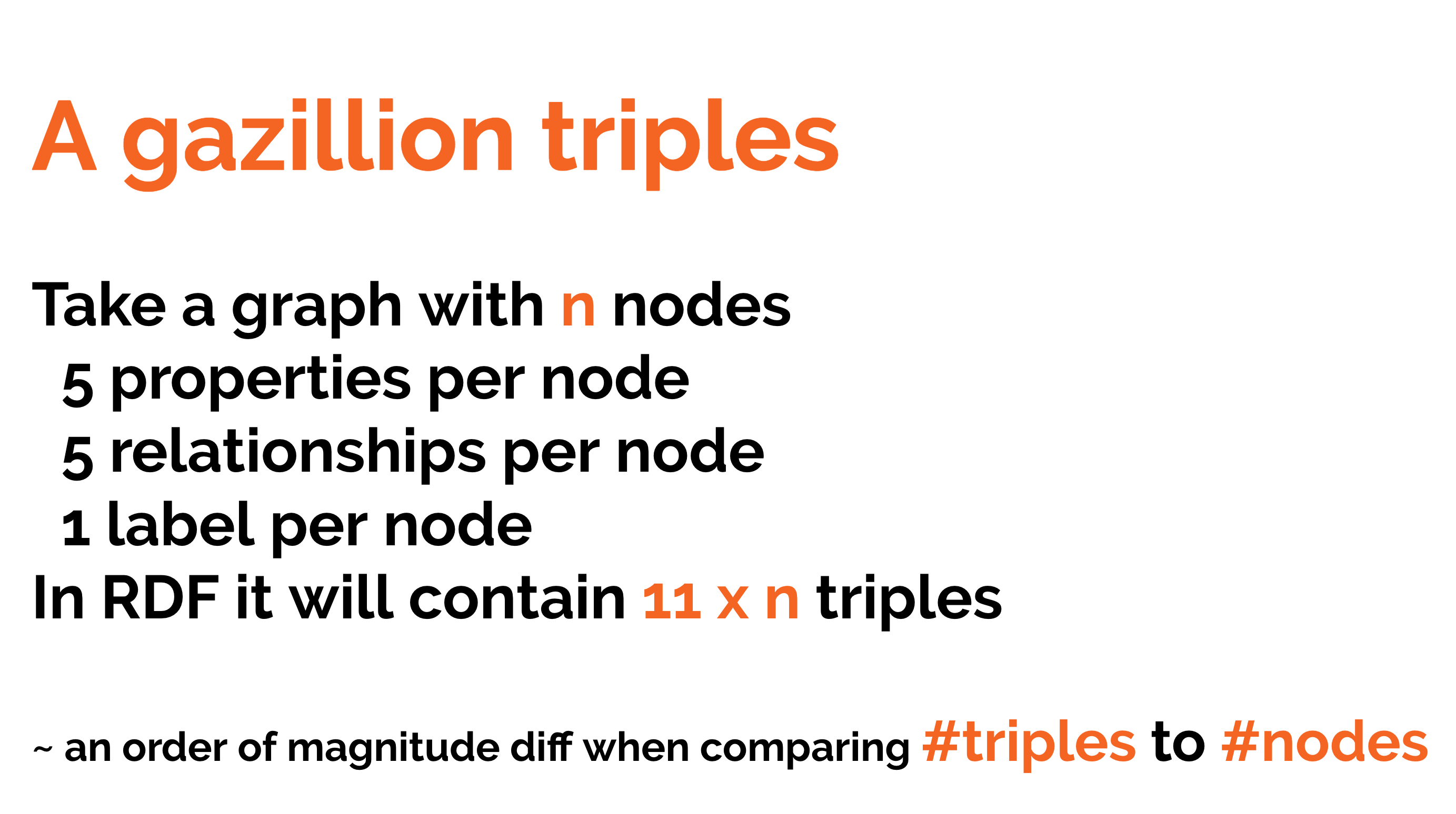
The raw import produces a graph with 18.8 million nodes and 101 million relationships. As usual, there is an order of magnitude more triples in the RDF graph than nodes in the LPG as discussed in the previous post.
I’ll start the analysis by getting some metrics on the imported dataset. This query will give us the avg/min/max/percentiles degree of the nodes in the graph:
MATCH (n)
WITH n, size((n)-[]-()) AS degree
RETURN AVG(degree), MAX(degree), MIN(degree),
 percentileCont(degree,.99) as `percent.99`,
 percentileCont(degree,.9999)as `percent.9999`,
 percentileCont(degree,.99999)as `percent.99999`;
+-------------------------------------------------------------------------------------+
| AVG(degree) | MAX(degree) | MIN(degree) | percent.99 | percent.9999 | percent.99999 |
+-------------------------------------------------------------------------------------+
| 5.377148198 | 9696290     | 0           | 20.0       | 205.0        | 8789.78792    |
+-------------------------------------------------------------------------------------+
We see that the average degree of the nodes in the graph is close to 5 but there are super dense nodes with up to 10 million (!) relationships. These dense nodes are a very small minority as we can see in the percentile information and they are due to specific modelling decisions that are OK in RDF but total anti-patterns when modelling a Property Graph. But don’t worry, we should be able to refactor the graph as I’ll show in the following section.
We also see from the MIN(degree) being zero in the previous query that there are some orphan nodes -not connected to any other node in the graph-. Let’s find more about them by running the following query (and the equivalent one for Organizations):
MATCH (n:ns7__Person) WHERE NOT (n)--()
RETURN count(n)
In the public dataset 34% of the Person entities are completely disconnected (this is 1.48 million out of a total of 4.4 million). The same happens with 5% of the Organizations (200K out of a total of 4.5mill).
Refactoring LPG antipatterns in the RDF graph
Nodes that could (should) be properties
In the RDF OpenPermID graph, there are a number of properties (hasPublicationStatus or hasGender in Persons or hasActivityStatus in Organizations) for which the value is either boolean style (active/inactive for hasActivityStatus) or have a very reduced set of values (male/female for hasGender). In the RDF graph, these values are modelled as resources instead of literals and they generate very dense nodes when imported into an LPG like Neo4j. Think of three or four million Person nodes with status active, all linked through the hasStatus relationship to one single node representing the ‘active’ status. The status -and the same goes for all the other properties mentioned before- can perfectly be modelled as node attributes (literal properties in RDF) without any loss of information so we’ll get rid of them with Cypher expressions like the following:
MATCH (x:ns7__Person)-[r:ns0__hasPublicationStatus]->(v)
SET x.ns0__publicationStatus = substring(v.uri,length('http://permid.org/ontology/common/publicationstatus'))
DELETE r
If we tried to run this on the whole PermID dataset it would involve millions of updates so we will want to batch it using APOC’s periodic commit procedure as follows:
CALL apoc.periodic.commit("
MATCH (x:ns7__Person)-[r:ns0__hasPublicationStatus]->(v)
WITH x,r,v LIMIT $limit
SET x.ns0__publicationStatus = substring(v.uri,length('http://permid.org/ontology/common/publicationstatus'))
DELETE r
RETURN COUNT(r)
", { limit : 50000});
I’ll apply the same transformation to the rest of the mentioned properties, you can see the whole script here (and you can run it too).
Nodes that are not needed
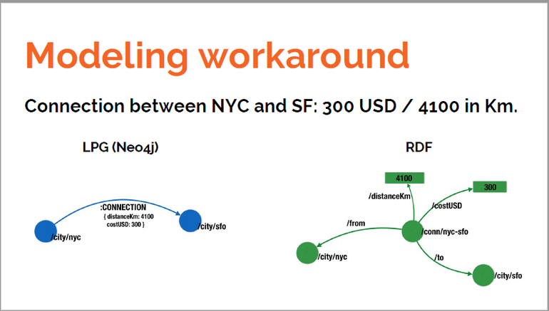
As I’ve discussed in previous articles and talks, in the LPG each instance of a relationship is uniquely identified and can have properties. This is not the case in RDF and in order to represent qualified relationships, they need to be reified as nodes (there are other options but I’m not going to talk about them here). Here is an example (that I used in a presentation a while ago) of what I’m talking about:
A very similar approach is used in OpenPermID to represent tenures in organizations. Tenures are modelled as resources in RDF (nodes in LPG) that contain information like the role and the start and end dates indicating its duration and they are connected to the person and the organization.
With the following refactoring, we will remove the intermediate (and unnecessary in an LPG) node representing the tenure and we will store all the information about it in a newly created relationship (:HOLDS_POSITION_IN) connecting directly the Person and the Organization. We are essentially transforming a graph like the green one in the previous diagram into another one like the blue one.
Here’s the Cypher that will do this for you:
MATCH (p)-[:ns7__hasTenureInOrganization]->(t:ns7__TenureInOrganization)-[:ns7__isTenureIn]->(o)
MERGE (p)-[hpi:HOLDS_POSITION_IN { ns0__hasPermId : t.ns0__hasPermId }]->(o) ON CREATE SET hpi+=t
DETACH DELETE t
As in the previous example, this is a heavy operation over the whole graph that will update millions of nodes and relationships so we will want to batch it in a similar way using apoc.periodic.commit. Remember that the complete script with all the changes is available here.
call apoc.periodic.commit("
MATCH (p)-[:ns7__hasTenureInOrganization|ns7__hasHolder]-(t:ns7__TenureInOrganization)-[:ns7__isTenureIn]->(o)
WITH p, t, o LIMIT $limit
MERGE (p)-[hpi:HOLDS_POSITION_IN { ns0__hasPermId : t.ns0__hasPermId }]->(o) ON CREATE SET hpi+=t
DETACH DELETE t
RETURN count(hpi)", {limit : 25000}
) ;
Ok, so we could go on with the academic qualifications, etc… but we’ll leave the transformations here for now. It’s time to start querying the graph.
Querying the graph
Path analysis
Let’s start with a classic: “What is the shortest path between…” I’ll use the last two presidents of the US for this example but feel free to make your choice of nodes. For our first attempt, we can be lazy and ask Neo4j to find a shortestPath between the two nodes that we can look up by name and surname. Here’s how:
MATCH p = shortestPath((trump:ns7__Person {`ns2__family-name` : "Trump", `ns2__given-name` : "Donald" })-[:HOLDS_POSITION_IN*]-(obama:ns7__Person {`ns2__family-name` : "Obama", `ns2__given-name` : "Barack" }))
RETURN p

This query returns one of the multiple shortest paths starting in Trump and ending in Obama and formed of people connected to organisations. The connections meaning that they hold or have held positions at such organisations at some point.
If we were doing this in a social/professional network platform to find an indirect connection (a path) to link two people via common friends/ ex-colleagues/etc, then the previous approach would be incomplete. And this is because if we want to be sure that two people have been sitting on the board of an organization at the same time, or held director positions at the same time, etc, we will have to check that there is a time overlap in their tenures. In our model, the required information is in the HOLDS_POSITION_IN relationship, which is qualified with two properties (from and to) indicating the duration of the tenure.
Let’s try to express this time-based constraint in Cypher: In a pattern like this one…
(x:Person)-[h1:HOLDS_POSITION_IN]->(org)<-[h2:HOLDS_POSITION_IN]-(y:Person)
…for x and y to know each other, there must be an overlap on the intervals defined by the from and to of h1 and h2. Sounds complicated? Nothing is too hard for the combination of Cypher + APOC.
MATCH p = shortestPath((trump:ns7__Person {`ns2__family-name` : "Trump", `ns2__given-name` : "Donald" })-[:HOLDS_POSITION_IN*]-(obama:ns7__Person {`ns2__family-name` : "Obama", `ns2__given-name` : "Barack" }))
WHERE all(x in filter( x in apoc.coll.pairsMin(relationships(p)) WHERE (startNode(x[0])<>startNode(x[1]))) WHERE
 not ( (x[0].to < x[1].from) or (x[0].from > x[1].to) )
)
return p
We are checking that every two adjacent tenures in the path -connecting two individuals to the same organization- do overlap in time. Even with the additional constraints, Neo4j only takes a few milliseconds to compute the shortest path.

In the first path visualization (and you’ll definitely find it too if you run your own data analysis) you may have noticed some of the Person nodes appear in yellow and with no name. This is because they have no properties other than the URI. The OpenPermID data dump seems to be incomplete and for some entities, it only includes the URI and the connections (ObjectProperties in RDF lingo) but is missing the attributes (the datatype properties). There are over 40K persons in this situation as we can see running this query:
MATCH (p)-[:HOLDS_POSITION_IN]->()
WHERE NOT p:ns7__Person
RETURN COUNT( DISTINCT p) AS count

╒═══════╕
│"count"│
╞═══════╡
│46139  │
└───────┘
And the symmetric one shows that also nearly 5K organizations have the same problem.
Luckily, the nodes in this situation have their URI, which is all we need to look them up in the PermID API. Let’s look at one random example: https://permid.org/1-34415693987. No attributes for this node, although we see that it has a number of :HOLDS_POSITION_IN connections to other nodes.
MATCH (r :Resource { uri : "https://permid.org/1-34413241385"})-[hpi:HOLDS_POSITION_IN]->(o)
RETURN *

Who is this person? Let’s get the data from the URI (available as HTML and as RDF):


So we now know that it represents Mr David T. Nish, effectively connected to the organisations we saw in the graph view. So we can fix the information gap by ingesting the missing triples directly from the API as follows:
call semantics.importRDF("https://permid.org/1-34413241385?format=turtle","Turtle",{})
This invocation of the importRDF procedure will pull the triples from the API and import them into Neo4j in the same way we did the initial data load.
It’s not clear to me why some random triples are excluded from the bulk download… Let’s run another example of path analysis with someone closer to me than the POTUSes. Let’s find the node in OpenPermID representing Neo4j.
MATCH (neo:ns3__Organization {`ns2__organization-name` : "Neo4j Inc"})
RETURN neo

If we expand neo Neo4j node in the browser we’ll find that the details of all the individuals connected to it are again not included in the bulk export dataset (all the empty yellow nodes connected to ‘Neo4j Inc’ through HOLDS_POSITION relationships), so let’s complete them in a single go with this fragment of Cypher calling semantics.importRDF for each of the incomplete Person nodes:
MATCH (neo:ns3__Organization {`ns2__organization-name` : "Neo4j Inc"})<-[:HOLDS_POSITION_IN]-(person)
WITH DISTINCT person
CALL semantics.importRDF(person.uri + "?format=turtle&access-token=","Turtle",{})
YIELD terminationStatus,triplesLoaded,extraInfo
RETURN *
Once we have the additional info in the graph, we can ask Neo4j what would be Emil’s best chance of meeting Mark Zuckerberg (why not?).
MATCH p = shortestPath((emil:ns7__Person {`ns2__family-name` : "Eifrem", `ns2__given-name` : "Emil" })-[:HOLDS_POSITION_IN*]-(zuck:ns7__Person {`ns2__family-name` : "Zuckerberg", `ns2__given-name` : "Mark" }))
WHERE all(x in filter( x in apoc.coll.pairsMin(relationships(p)) WHERE (startNode(x[0])<>startNode(x[1]))) WHERE NOT ( (x[0].to < x[1].from) or (x[0].from > x[1].to) ) )
RETURN p

Nice! Now finally, and just for fun, return the same results as a description in English of what this path looks like. All we need to do is add the following transformation to the previous path query. Just replace the return with the following two lines:
UNWIND filter( x in apoc.coll.pairsMin(relationships(p)) WHERE (startNode(x[0])<>startNode(x[1]))) as match
RETURN apoc.text.join(collect(startNode(match[0]).`ns2__family-name` + " knows " + startNode(match[1]).`ns2__family-name` + " from " + endNode(match[0]).`ns2__organization-name`),", ") AS explanation
And here’s the result:
Eifrem knows Treskow from Neo4j Inc, Treskow knows Earner from Space Ape Games (UK) Ltd, Earner knows Breyer from Accel Partners & Co Inc, Breyer knows Zuckerberg from Facebook Inc.
Industry / Economic Sector classification queries
Another interesting analysis is the exploration of the industry/economic sector hierarchy. The downside is that only 8% of the organizations in the dataset are classified according to it.
Here is, however, a beautiful bird’s eye view of the whole economic sector taxonomy where we can see that industry sub-taxonomies are completely disjoint between each other and the two richest hierarchies are the one for Consumer Cyclicals and Industrials :
MATCH (n:ns10__EconomicSector)<-[b:ns6__broader*]-(c)
RETURN *

And a probably more useful detailed view of the Telecoms sector:
MATCH (n:ns10__EconomicSector)<-[b:ns6__broader*]-(c)
WHERE n.ns9__label = "Telecommunications Services"
RETURN *

Instrument classification queries
Similar to the industries and economic sectors, instruments issued by organizations are classified in a rich hierarchy of asset categories. The problem again is that in the public dataset only 2% (32 out of nearly 1400) of the asset categories have instruments in them. This makes the hierarchy limited in use. Let’s run a couple of anlaytic queries on the hierarchy.
The following table shows the top level asset categories that have at least an instrument or a subcategory in them:

And here is the Cypher query that produces the previous results
MATCH (ac:ns5__AssetClass)
WHERE NOT (ac)-[:ns6__broader]->() //Top level only
WITH ac.ns9__label as categoryName, size((ac)<-[:ns6__broader*]-()) as childCategoryCount, size((ac)<-[:ns6__broader*0..]-()<-[:ns5__hasAssetClass]-(:ns5__Instrument)) as instrumentsInCategory  WHERE childCategoryCount + instrumentsInCategory > 0
RETURN categoryName, childCategoryCount, instrumentsInCategory
ORDER BY childCategoryCount + instrumentsInCategory DESC
The instruments in the public DB are all in under the “Equities” category, and within this category, they are distributed as follows (only top 10 shown, remove limit in the query to see all):

Here’s the Cypher query that produces the previous results.
MATCH (:ns5__AssetClass { ns9__label : "Equities"})<-[:ns6__broader*0..]-(ac)
WITH ac.uri as categoryId, ac.ns9__label as categoryName, size((ac)<-[:ns5__hasAssetClass]-(:ns5__Instrument)) as instrumentsInCategory
RETURN categoryName, instrumentsInCategory
ORDER BY instrumentsInCategory DESC LIMIT 10
To finalise the analysis of the asset categories, a visualization of the “Equities” hierarchy with the top three (by number of instruments in the dataset) highlighted.

Global queries and integration with BI tools
Cypher queries on the graph can return rich structures like nodes or paths, but they can also produce data frames (data in tabular form) that can easily be used by standard BI tools like Tableau, Qlik, Microstrategy and many others to create nice charts. The following query returns the ratio of women holding positions at organizations both by country and economic sector.
MATCH (c:Country)<-[:ns3__isIncorporatedIn|ns4__isDomiciledIn]-(o)<-[:HOLDS_POSITION_IN]-(p) OPTIONAL MATCH (o)-[:ns3__hasPrimaryEconomicSector]->(es)
WITH c.Country AS country, coalesce(es.ns9__label,'Unknown') AS economicSector, size(filter(x in collect(p) where x.ns2__gender = "female")) AS femaleCount, count(p) AS totalCount
RETURN country, economicSector, femaleCount, totalCount, femaleCount*100/totalCount as femaleRatio
Here is an example of how this dataset can be used in Tableau (tableau can query the Neo4j graph directly using Cypher via the Neo4j Tableau WDC).
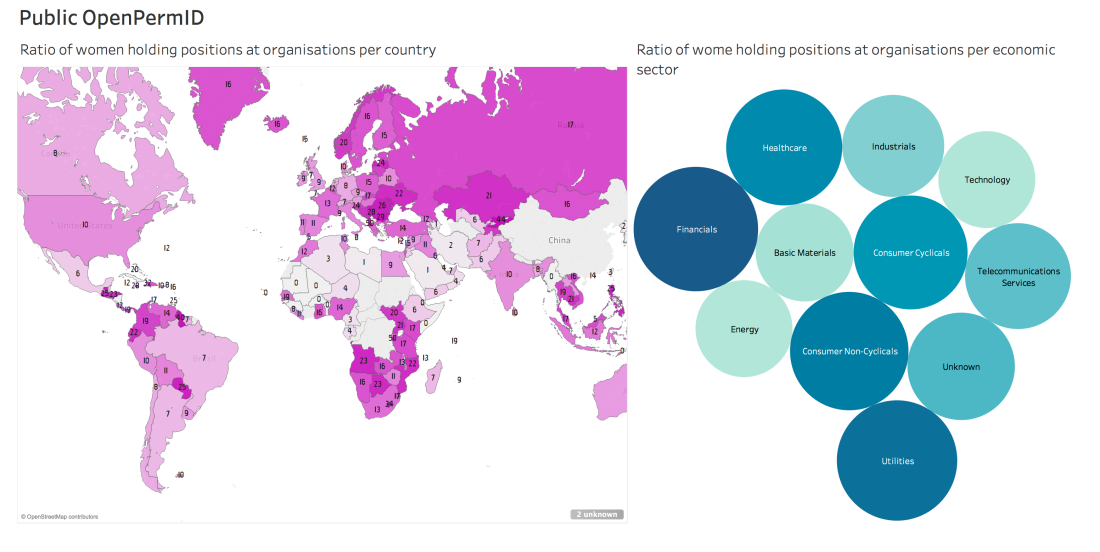
According to the public OpenPermID dataset, the top three countries ranked by ratio of women holding positions at organisations are Burundi, Albania and Kyrgyzstan. Interesting… not what I was expecting to be perfectly honest, and definitely not aligned with other analysis and sources. The chart to the right shows that women are evenly distributed across economic sectors which sounds plausible.
Well, I would expect you to be at least as sceptical as I am about these results, and I believe it has again to do with the fact that the dataset seems to be incomplete, so please do not take this as anything more than a data integration / manipulation exercise.
Other data quality issues
Entity duplication
While running some of the queries, I noticed some duplicate nodes. Here is an example of what I mean, the one and only duplicate Barak Obama.
MATCH (obama:ns7__Person)
WHERE obama.`ns2__family-name` = "Obama" AND
      obama.`ns2__given-name` = "Barack"
RETURN obama

One of the Obama nodes (permID: 34414148146) seems to connect to the organizations he’s held positions in and the other one (permID: 34418851840) links to his academic qualifications. Maybe two sources (academic + professional) have been combined in OpenPermID but not integrated completely yet?
Here’s how Cypher can help detecting these complex patterns proving why graph analysis is extremely useful for entity resolution. The following query (notice it’s quite a heavy one) will get you some 30K instances of this pattern (which means at least 2x as many nodes will be affected). I’ve saved the likely duplicates in the dupes.csv file in this directory.
MATCH (p1:ns7__Person)
WHERE (p1)-[:ns7__hasQualification]->() AND NOT (p1)-[:HOLDS_POSITION_IN]->()
WITH DISTINCT p1.`ns2__given-name` AS name, p1.`ns2__family-name` AS sur, coalesce(p1.`ns2__additional-name`,'') AS add
MATCH (p2:ns7__Person)
WHERE p2.`ns2__family-name` = sur AND
p2.`ns2__given-name` = name AND
coalesce(p2.`ns2__additional-name`,'') = add AND
(p2)-[:HOLDS_POSITION_IN]->() AND
NOT (p2)-[:ns7__hasQualification]->()
RETURN DISTINCT name, add, sur
Default dates
If you’re doing date or interval computations, keep an eye also on default values for dates because you will find both nulls an the famous 1st Jan 1753 (importing data from SQL Server?). Make sure you deal with either case in your Cypher queries.
Here’s the Cypher query you can use to profile the dates in the HOLD_POSITION_IN relationship, showing at the top of the frequency list the two special cases mentioned.
MATCH (:ns7__Person)-[hpi:HOLDS_POSITION_IN]->()
RETURN hpi.ns0__from AS fromDate, count(hpi) AS freq
ORDER BY freq DESC

Your data in Neo4j serialized as RDF
So, going back to the title of the post, if “Neo4j is your RDF store”, then you should be able to serialize your graph as RDF. The neosemantics extension not only helped us in the ingestion of the RDF, but also gives us a simple way to expose the graph in Neo4j as RDF. And the output is identical to the one in the PermID API. Here is, as an example, the RDF description generated directly from Neo4j of Dr Jim Webber, our Chief Cientist:

Even more interesting, we can have the result of a Cypher query serialized as RDF. Here’s an example producing the graph of Dr. Weber’s colleagues at Neo4j.

Takeaways
Once again we’ve seen how straightforward it is to import RDF data into Neo4j. Same as serializing a Neo4j graph as RDF. Remember, RDF is a model for data exchange but does not impose any constraint on where/how the data is stored.
I hope I’ve given a nice practical example of (1) how to import a medium-size RDF graph into Neo4j, (2) transform and enrich it using Cypher and APOC and finally (3) query it to benefit from Neo4j’s native graph storage.
Now download Neo4j if you have not done it yet, check out the code from GitHub and give it a try! I’d love to hear your feedback.

Can you provide more information on how to run the script please?
LikeLike
Well, there’s not much about it.
I assume you have neo4j installed (plus neosemantics).
All you need to do is download the permid data and run the scripts in the browser or in the cypher shell.
Here’s the link to the cypher scripts: https://github.com/jbarrasa/openpermid2neo4j
LikeLike
Is there any way to export the whole dataset as RDF?
LikeLike
Sure, you just need to write the cypher query that returns the portion of the graph you want to export (or the whole graph if that’s what you want) and send it to the /rdf/cypheronrdf endpoint. (Or /rdf/cypher depending on the type of graph you have in Neo4j). Check the manual here: http://jbarrasa.github.io/neosemantics/
Also, in this particular example the data was originally RDF, so you basically already have it as RDF 😉
LikeLike
Thank You for the great posts, I really benefited from them. I am working with RDF and Neo4j (+nsmntx) at the moment. I have imported my model (RDF/XML) that contains around 5 million nodes, using “CALL n10s.rdf.import.fetch ()”. I queried it using Cypher, I had to execute the same query for 325094 nodes looking for their location. Neo4j took over 10h to execute all of these queries with the mean execution time being 252.13ms. It seems way too much. I worked also with GraphDB and needed only 6min for the same use case. Any idea why Neo4j needed so much more time? I would appreciate Your help so much, I wouldn’t like to get a wrong conclusion, maybe I didn’t optimize something. I have a commercial version of Neo4j server and measured the time using Java time in Eclipse IDE.
Thanks in advance!
LikeLike
Hi Amila, thanks for your interest and thanks for sharing your experience.
We should definitely be able to improve the numbers you’re describing.
But it’s difficult to tell without having a bit more context.
Would you be open to sharing the dataset and queries you’ve used in your experiment?
The best way would be via Github but if that is not possible you can email me at jesus dot barrasa at neo4j dot com.
Cheers,
JB.
LikeLike
Thank You so much for the fast reply. Unfortunately, I do not own the dataset, I was just granted permission to use it for research purposes. I can share my queries and code with You and some statistics regarding the model. I will send more detailed data to Your e-mail address. Thank You for the interest, it means a lot to me. Best regards, Amila
LikeLike